Separable First Order Differential Equations - Basic Introduction
TLDRThis video script presents a comprehensive guide on solving differential equations through the method of separating variables. It walks through multiple examples, demonstrating how to isolate variables, integrate both sides of the equation, and apply initial conditions to find particular solutions. The script covers a range of scenarios, from basic equations like dy/dx = x^2/y^2 to more complex ones involving functions like y' = x*y and dy/dx = y^2 + 1. Each step is clearly explained, making the content accessible for learners to grasp the fundamental concepts and techniques of differential equations.
Takeaways
- 📚 The video focuses on solving differential equations using the method of separating variables.
- 🔍 To separate variables, place all y terms on one side of the equation and all x terms on the other side.
- 🧠 The first example involves the differential equation d y/d x = x²/y², which is solved by cross-multiplying and integrating both sides.
- 🌟 The antiderivative of y² is y³/3 and the antiderivative of x² is x³/3, with an additional constant C.
- 📈 The general solution for the first example is y³ = x³ + C, and by taking the cube root of both sides, y = (x³ + C)^(1/3).
- 🔑 A particular solution is found by using an initial condition; for y(1) = 2, the constant C is determined to be 7.
- 📝 In the second example, y' = x*y, the separation of variables is done by multiplying both sides by dx and dividing by y.
- 🤔 The natural log and exponentiation are used to solve the second example, resulting in the general solution y = C * e^(1/2 * x²).
- 📌 The particular solution for the second example, given y(0) = 5, is found by setting C to 5, resulting in y = 5 * e^(1/2 * x²).
- 🧩 The third example involves the differential equation d y/d x = y² + 1, and the initial condition y(1) = 0.
- 👉 The general solution for the third example is y = tan(x + C), and by using the initial condition, a particular solution is y = tan(x - 1).
Q & A
What is the main method discussed in the video for solving differential equations?
-The main method discussed in the video for solving differential equations is by means of separating variables.
How do you separate variables in the given example where dy/dx = x^2/y^2?
-To separate variables in the given example, you cross multiply to obtain y^2 dy = x^2 dx, then integrate both sides to get ∫y^2 dy = ∫x^2 dx, resulting in y^3/3 = x^3/3 + C, where C is the constant of integration.
What is the general solution for the differential equation dy/dx = x^2/y^2?
-The general solution for the differential equation dy/dx = x^2/y^2 is y^3 = x^3 + C, where C is a constant.
How do you find a particular solution given an initial condition?
-To find a particular solution given an initial condition, you substitute the initial condition (x and y values) into the general solution and solve for the constant of integration, C.
What is the initial condition used in the example to find the particular solution for dy/dx = x^2/y^2?
-The initial condition used in the example to find the particular solution for dy/dx = x^2/y^2 is y(1) = 2.
How do you solve the differential equation y' = x*y, given the initial condition y(0) = 5?
-To solve the differential equation y' = x*y with the initial condition y(0) = 5, you separate variables by multiplying both sides by dx and dividing by y, then integrate both sides to obtain ln(y) = (1/2)x^2 + C. The general solution is y = e^((1/2)x^2 + C), and by substituting x = 0 and y = 5, you find C = 5, resulting in the particular solution y = 5e^((1/2)x^2).
What is the significance of the natural logarithm (ln) and exponentiation (e) in solving the second example differential equation?
-In solving the second example differential equation, the natural logarithm (ln) and exponentiation (e) are used to transform the equation into a form where the exponents can be equated, allowing for the separation of variables and the determination of the general solution.
How do you find the general solution for the differential equation dy/dx = y^2 + 1?
-To find the general solution for the differential equation dy/dx = y^2 + 1, you first separate the variables by dividing both sides by y^2 + 1 and integrating to obtain arctan(y) = x + C. The general solution is then y = tan(x + C).
What is the particular solution for the differential equation dy/dx = y^2 + 1 when y(1) = 0?
-The particular solution for the differential equation dy/dx = y^2 + 1 when y(1) = 0 is found by setting x = 1 and y = 0 in the general solution y = tan(x + C). This results in tan(C) = 0, which implies C = 0. Thus, the particular solution is y = tan(x).
What is the role of the inverse tangent function (arctan) in solving the third example differential equation?
-The inverse tangent function (arctan) is used in solving the third example differential equation because its derivative is 1/(1 + x^2), which matches the form of the given differential equation after separation of variables. This allows for the integration of the equation to find the general solution.
How do you handle the constant of integration (C) when finding particular solutions?
-When finding particular solutions, the constant of integration (C) is determined by substituting the given initial condition into the general solution and solving for the value of C that makes the equation true at the initial point.
What is the significance of taking the cube root of both sides in the general solution of the first example?
-Taking the cube root of both sides in the general solution of the first example simplifies the equation by reducing the power of y and x from three to one, resulting in a more manageable form of the solution, y = (x^3 + C)^(1/3).
Outlines
📚 Solving Differential Equations by Separating Variables
This paragraph introduces the method of solving differential equations by separating variables. It begins with an example problem where the equation is d y/d x = x^2/y^2. The process involves separating the variables to have y variables on one side and x variables on the other, then integrating both sides to find the antiderivative. The general solution is derived as y^3 = x^3 + 3c, and a particular solution is found by applying an initial condition y(1) = 2, leading to the solution y = (cube root of (x^3 + 7)). Another example is presented where y' = x*y, with an initial condition y(0) = 5, and the solution is found by separating the variables and applying the initial condition, resulting in y = 5e^((1/2)x^2). The explanation emphasizes understanding the process of separating variables and applying initial conditions to find particular solutions.
🔢 Manipulating Exponents and Logarithms in Differential Equations
This paragraph discusses the manipulation of exponents and logarithms in the context of differential equations. It starts with an example where y' = x*y and the initial condition is y(0) = 5. The process involves separating the variables and integrating both sides. The antiderivative of the left side is the natural log of y, and the right side becomes x^2/2 + c. By applying the initial condition, the constant c is found to be 5. The explanation then moves to another problem where d y/d x = y^2 + 1, with the initial condition y(1) = 0. The solution involves finding the antiderivative of the given equation and applying the initial condition to find the constant c, which turns out to be -1, leading to the particular solution y = tan(x) - 1. The paragraph emphasizes the importance of understanding how to handle exponents and logarithms when solving differential equations.
🌟 Applying Trigonometric Functions to Differential Equations
The final paragraph of the script focuses on the application of trigonometric functions in solving differential equations. The example given is d y/d x = y^2 + 1 with an initial condition y(1) = 0. The method involves separating the variables and integrating, leading to the antiderivative of the left side being the inverse tangent of y, and the right side being x + c. By applying the initial condition, the constant c is determined to be -1, resulting in the particular solution y = tan(x) - 1. The paragraph highlights the use of trigonometric identities and the process of finding particular solutions from a general solution by applying given initial conditions.
Mindmap
Keywords
💡Differential Equations
💡Separating Variables
💡Integration
💡Antiderivatives
💡Constants
💡Initial Conditions
💡Particular Solution
💡General Solution
💡Inverse Tangent
💡Natural Logarithm
💡Exponential Functions
Highlights
The video focuses on solving differential equations by separating variables, a fundamental technique in differential calculus.
The first example provided involves the equation dy/dx = x^2/y^2, which is a basic form of a separable differential equation.
To separate variables, the instruction is to have y-related terms on one side and x-related terms on the other, resulting in an equation ready for integration.
After separating variables, the next step is to integrate both sides of the equation, leading to the antiderivatives of the functions involved.
The antiderivative of y^2 is y^3/3, and the antiderivative of x^2 is x^3/3, with the addition of a constant term C to account for the integration.
The general solution of the first example is y^3 = x^3 + C, which can be further simplified by taking the cube root of both sides.
A particular solution is found by using an initial condition; in the example, y(1) = 2, which leads to solving for the constant C.
The second example involves the differential equation y' = x*y, with an initial condition y(0) = 5, providing a point (0, 5) to find the particular solution.
By multiplying both sides of the second equation by dx and dividing by y, the equation is rearranged to 1/y dy = x dx, leading to the natural logarithm of y.
The general solution for the second example is y = C * e^(x^2/2), derived by equating the exponents of e after finding the antiderivative of both sides.
Using the initial condition y(0) = 5, the constant C is found to be 5, resulting in the particular solution for the second example.
The third example given is dy/dx = y^2 + 1, with an initial condition y(1) = 0, which is used to find both the general and particular solutions.
The third example involves dividing both sides by y^2 + 1 and integrating to find the inverse tangent of y as the antiderivative.
The general solution for the third example is y = tan(x + C), where the constant C is determined by the initial condition.
By using the initial condition y(1) = 0, the particular solution is found to be y = tan(x - 1), with C being negative one.
The video demonstrates the importance of understanding the relationship between derivatives and antiderivatives in solving differential equations.
The method of separating variables is shown to be effective in finding both general and particular solutions to first-order differential equations.
The video provides a step-by-step approach to solving differential equations, making it accessible for learners at various levels of mathematical understanding.
The practical application of these methods can be seen in fields such as physics and engineering, where differential equations are commonly used to model systems.
The video emphasizes the use of initial conditions to find particular solutions, which is crucial in real-world problem-solving scenarios.
The transcript showcases the mathematical process of transforming a differential equation into a more manageable form through separation of variables and integration.
Transcripts
Browse More Related Video

AP Calculus AB Crash Course Day 5 - Integration and Differential Equations
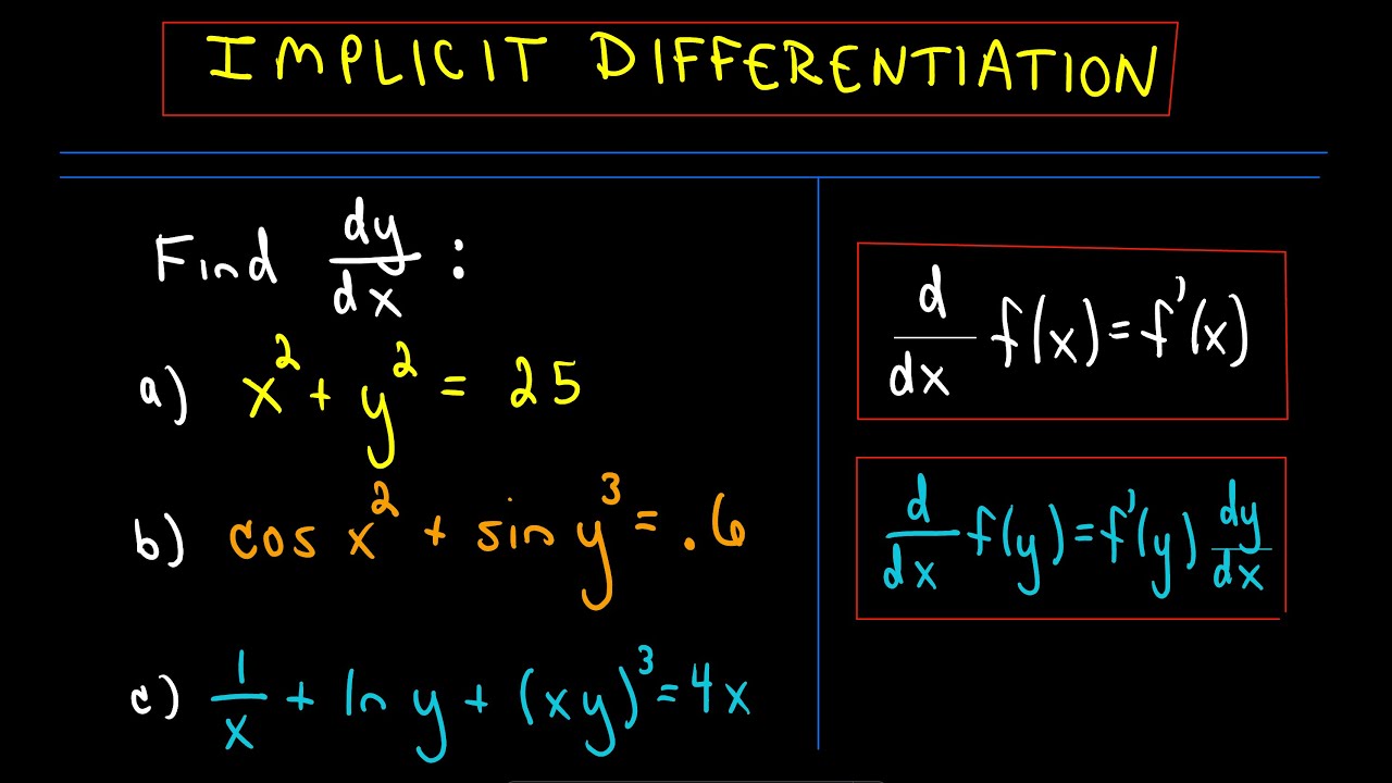
Implicit Differentiation for Calculus - More Examples, #1

Euler's Method Differential Equations, Examples, Numerical Methods, Calculus
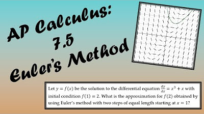
AP Calculus BC Lesson 7.5
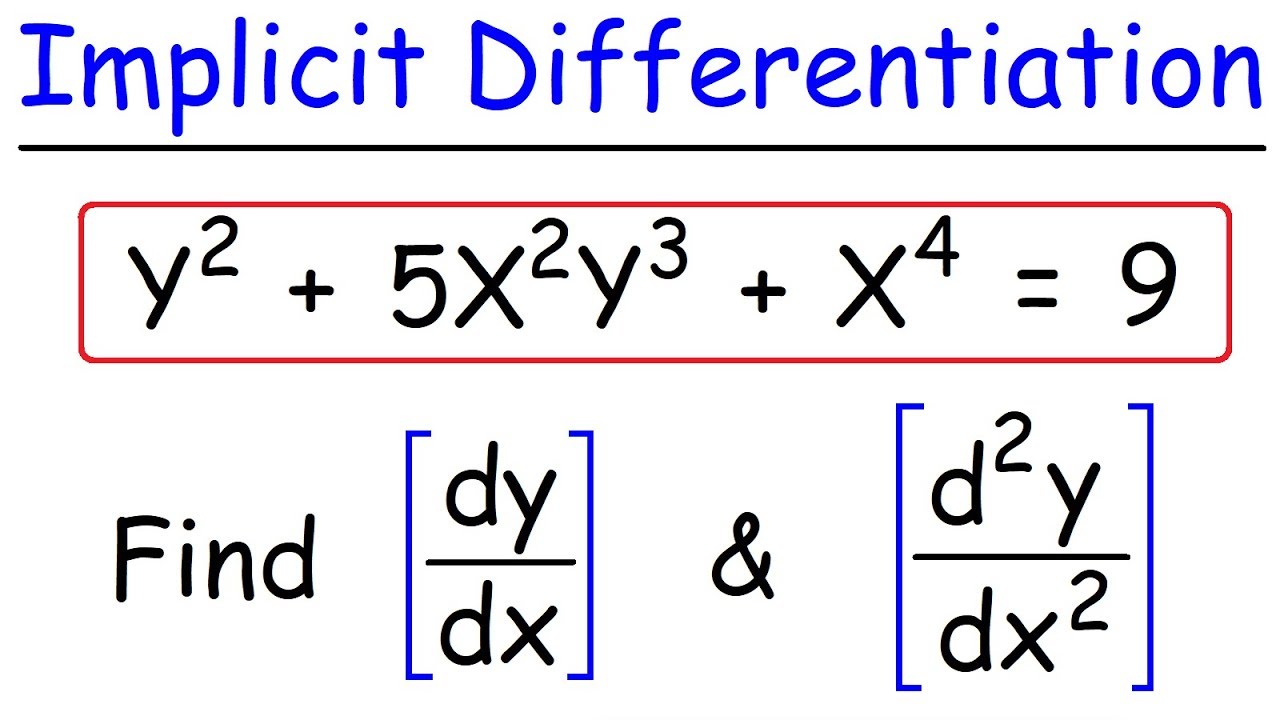
Implicit Differentiation - Find The First & Second Derivatives
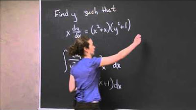
Differential Equation | MIT 18.01SC Single Variable Calculus, Fall 2010
5.0 / 5 (0 votes)
Thanks for rating: