Probability Exponential Distribution Problems
TLDRThis video explains how to solve probability exponential distribution problems, focusing on a specific example involving the lifespan of laptops produced by Company XYZ. It shows step-by-step how to calculate the rate parameter lambda, write the probability density function, find the probabilities that a laptop will last less than 3 years or more than 10 years, and determine the probability a laptop will last between 4 and 7 years. Visual representations accompany the explanations. This covers the basics of working with the exponential distribution in a probability context.
Takeaways
- 😀 The rate parameter lambda is calculated as 1 over the average lifespan
- 👨🏫 The probability density function (PDF) uses lambda and the exponential e^(-lambda*x)
- 📈 The PDF graph starts high on the y-axis and decreases over time
- 💡 To find P(X < x), use the formula: 1 - e^(-lambda*x)
- 🔢 To find P(X > x), use the formula: e^(-lambda*x)
- 😕 To find P(a < X < b), take P(X < b) - P(X < a)
- 📊 Visualizing areas under the PDF curve helps solve probability questions
- ✏️ Calculating step-by-step is key - don't skip directly to the final answer!
- 🤓 Understanding and applying the correct formulas is critical
- 🎥 The video covers basic exponential distribution probability problems
Q & A
What is the formula used to calculate the rate parameter lambda?
-The rate parameter lambda is calculated using the formula: lambda = 1/mu, where mu is the average lifespan. In this example, mu = 5 years, so lambda = 1/5 = 0.2 per year.
What is the probability density function for the laptop lifespan distribution?
-The probability density function is: f(X) = lambda * e^(-lambda * X) = 0.2 * e^(-0.2X)
What is the probability that a laptop will last less than 3 years?
-The probability is calculated using: P(X < 3 years) = 1 - e^(-lambda * X) = 1 - e^(-0.6) = 0.4512 or 45.12%
What does the y-intercept represent on the probability density function graph?
-The y-intercept represents the value of the probability density function when X = 0. In this case, it is equal to the rate parameter lambda = 0.2.
What is the probability that a laptop will last more than 10 years?
-P(X > 10 years) = e^(-lambda * X) = e^(-0.2 * 10) = e^(-2) = 0.1353 or 13.53%
How do you calculate the probability that the laptop lifespan is between 4 and 7 years?
-Take the difference between P(X < 7) and P(X < 4). Visually this represents the area under the probability density curve between X = 4 and X = 7.
What assumption is being made about the laptop lifespan distribution?
-It is assumed the laptop lifespan follows an exponential distribution, which models time between events in a Poisson process with a constant event rate.
What are some characteristics of the exponential distribution?
-The exponential distribution has a constant failure rate and models time between events in a Poisson process. It is often used to model the lifespan of electronic components.
Why is the exponential distribution useful for modeling laptop lifespan?
-The constant failure rate matches typical reliability characteristics of electronic components. Also, the distribution is memoryless, meaning the future lifespan does not depend on past usage.
What other variables could impact the predicted laptop lifespan distribution?
-Other factors like manufacturing variability, model differences, and usage patterns could alter the true lifespan distribution. More data and a statistical analysis would provide greater precision.
Outlines
📊 Calculating Parameters and Graphing the Probability Density Function
This paragraph calculates the rate parameter lambda for the exponential distribution of laptop lifespan based on the average lifespan. It then writes the probability density function with lambda and graphs it, showing how it decreases over time. It also calculates the y-intercept.
😯 Finding Probabilities Using the Distribution
This paragraph shows how to find the probability a laptop lasts less than 3 years using the area under the curve. It also shows how to find the probability a laptop lasts more than 10 years. Finally, it calculates the probability a laptop lasts between 4 and 7 years using the difference in areas.
👋 Concluding the Video
This closing paragraph thanks viewers for watching the video and invites them to subscribe to the channel.
Mindmap
Keywords
💡probability density function
💡exponential distribution
💡rate parameter
💡area under the curve
💡probability formula
💡mean lifetime
💡discrete intervals
💡cumulative probability
💡exponential decay
💡probability density curve
Highlights
The rate parameter lambda is calculated as 1 over the average lifespan, which is 1/5 = 0.2 years^-1
The probability density function (PDF) is f(x) = lambda * e^(-lambda * x), where lambda = 0.2
The PDF graph starts at y-intercept 0.2 and decreases over time
The probability X < 3 years is calculated using the CDF formula P(X < x) = 1 - e^(-lambda * x)
The probability X > 10 years is calculated using P(X > x) = e^(-lambda * x)
To find P(4 < X < 7), take the difference between P(X < 7) and P(X < 4)
P(X < 7) is calculated using the CDF formula 1 - e^(-lambda * x)
P(X < 4) is calculated similarly using the CDF formula
Take the difference between P(X < 7) and P(X < 4) to get the final probability
There is a 20.3% probability a laptop lasts between 4 and 7 years
Exponential distributions are used to model random events over time
The CDF formula calculates left-tail probabilities
The complementary CDF formula calculates right-tail probabilities
Subtracting CDF values gives probabilities for value ranges
These formulas allow solving a variety of exponential distribution problems
Transcripts
Browse More Related Video
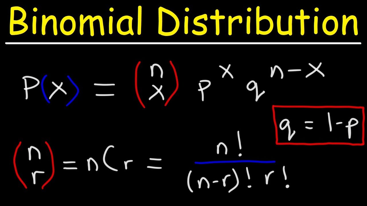
Finding The Probability of a Binomial Distribution Plus Mean & Standard Deviation
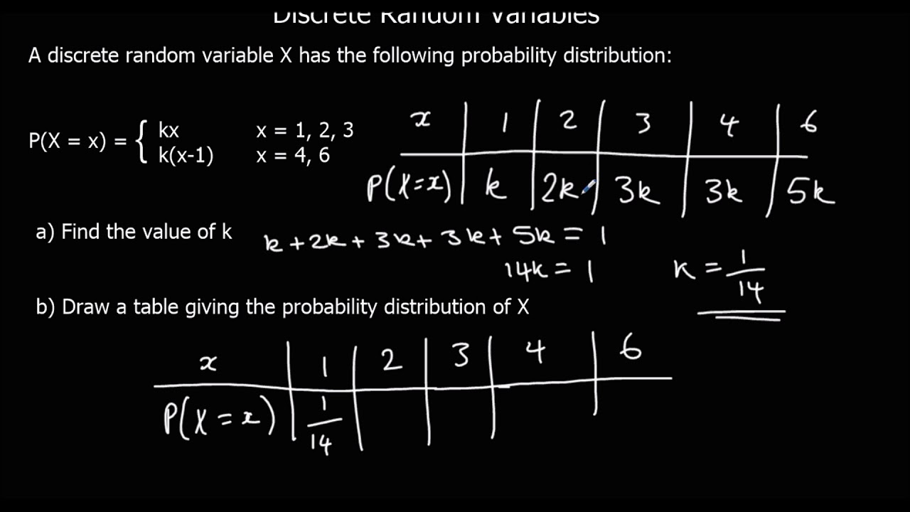
Discrete Random Variables

Probabilities from density curves | Random variables | AP Statistics | Khan Academy

Data Science & Statistics Tutorial: The Poisson Distribution
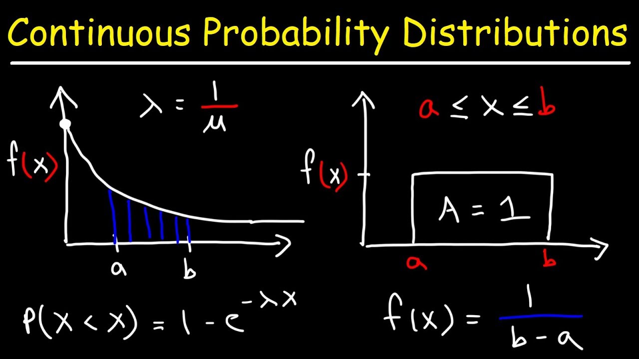
Continuous Probability Distributions - Basic Introduction
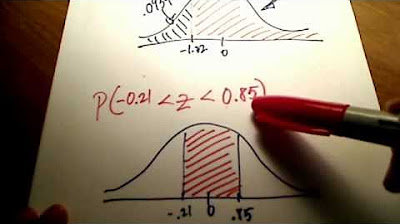
Stats: Finding Probability Using a Normal Distribution Table
5.0 / 5 (0 votes)
Thanks for rating: