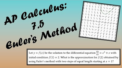
Euler's Method Differential Equations, Examples, Numerical Methods, Calculus
TLDRThe video script presents a detailed explanation of Euler's method for approximating solutions to differential equations. It begins with a simple function y = x^2 and its derivative dy/dx = 2x, using an initial condition of (1,1) and a step size of 0.1 to estimate y at x = 1.5. The process involves creating a table for iterative calculations, correcting the slope at each step to improve accuracy over the tangent line approximation. The script also compares Euler's method to the tangent line approximation, demonstrating the former's superior accuracy through a graphical representation. Finally, the script challenges viewers to apply Euler's method to a different differential equation, y' = x + 2y, with an initial condition of y(2) = 3, and to estimate y at x = 2.5 using the same step size, providing a comprehensive guide to understanding and applying this mathematical technique.
Takeaways
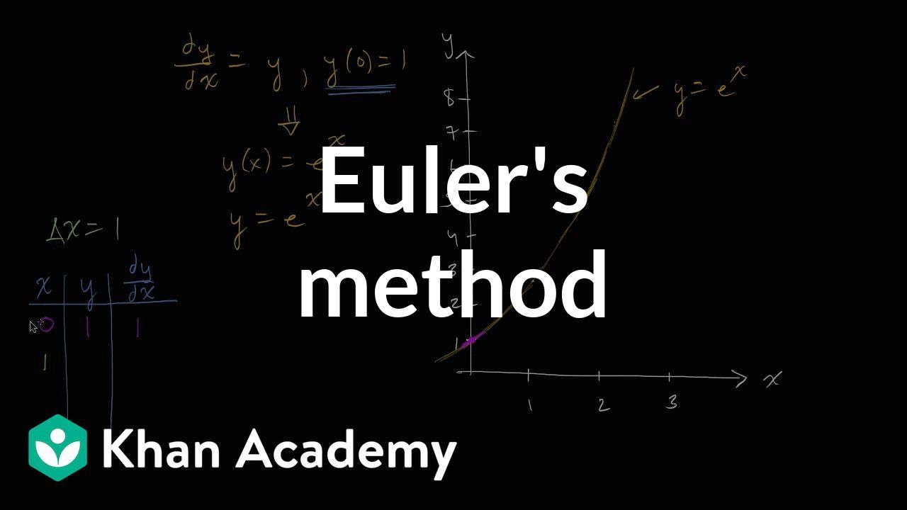
- 📚 Euler's method is used to approximate the solution of a differential equation by taking small steps and adjusting the slope at each step.
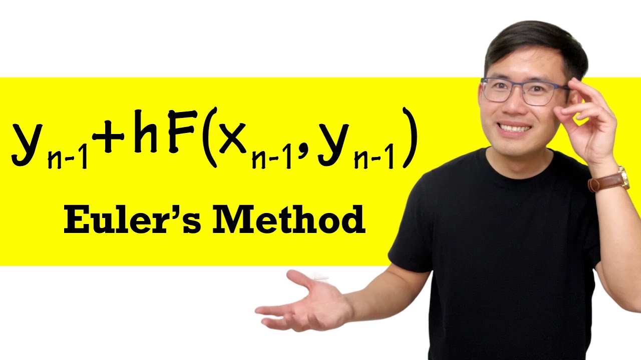
- 🔍 The formula for Euler's method is y_{n+1} = y_n + h \cdot f'(x, y), where h is the step size and f'(x, y) is the derivative of the function.
- 📈 The accuracy of Euler's method increases with a smaller step size h.
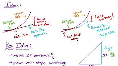
- 📉 Euler's method provides a better approximation than the tangent line approximation because it includes course correction at each step.
- 🧮 To apply Euler's method, create a table with columns for n, x_n, y_n, and the actual value of the function at each step.
- 📌 The initial condition provides the starting point (x_0, y_0) for the calculation.
- 🤓 The derivative f'(x) or f'(x, y) is used to determine the slope of the tangent line at each step.
- 🚀 Euler's method involves iterative calculation of y values as x increases by increments of h.
- 📊 By plotting the function and the tangent lines, one can visualize how Euler's method adjusts the path to better approximate the curve.
- 🤖 For a more complex differential equation y' = x + 2y, the method still applies, but now f'(x, y) = x + 2y.
- 🔗 The relationship between the equation and the graph is that the slope of the line connecting two points on the graph is given by f'(x), showing how the function changes over small intervals.
Q & A
What is Euler's method used for?
-Euler's method is used to approximate the solution of a differential equation.
What is the differential equation used in the video example?
-The differential equation used in the video example is dy/dx = 2x.
What is the initial condition given for the first example in the video?
-The initial condition given for the first example is (x, y) = (1, 1).
What is the step size (h) used in the first example?
-The step size (h) used in the first example is 0.1.
How does Euler's method differ from the tangent line approximation?
-Euler's method is similar to the tangent line approximation but includes course correction at every step size (h), which leads to a better approximation of the solution.
What is the estimated value of y when x is 1.5 using Euler's method in the first example?
-The estimated value of y when x is 1.5 using Euler's method is approximately 2.2.
What is the exact value of y when x is 1.5 according to the original function y = x^2?
-The exact value of y when x is 1.5 according to the original function y = x^2 is 2.25.
How does decreasing the step size (h) affect the accuracy of Euler's approximation?
-Decreasing the step size (h) increases the accuracy of Euler's approximation.
What is the relationship between the differential equation and the graph when using Euler's method?
-The relationship between the differential equation and the graph is that the slope of the line connecting two consecutive points on the graph is given by f'(x), which is the derivative used in Euler's method.
What is the differential equation and initial condition used in the second example of the video?
-The differential equation used in the second example is y' = x + 2y, with the initial condition y(2) = 3.
What is the estimated value of y when x is 2.5 using Euler's method in the second example?
-The estimated value of y when x is 2.5 using Euler's method in the second example is approximately 9.08.
Why is it important to calculate f'(x, y) for each step in Euler's method?
-Calculating f'(x, y) for each step is important because it provides the slope of the tangent line at the current point, which is then used to estimate the next point on the solution curve.
Outlines
📐 Introduction to Euler's Method for Differential Equations
The video begins with an introduction to using Euler's method to approximate solutions to differential equations. A simple function y = x^2 is chosen for demonstration, with the differential equation dy/dx = 2x. The goal is to estimate the value of y when x = 1.5. Euler's method is compared to the tangent line approximation, with an emphasis on its iterative nature, using a step size (h) of 0.1 and starting from the initial condition (1,1). The formula for Euler's method is provided, and the process is illustrated through a step-by-step calculation for each value of n from 0 to 5, adjusting the x and y values accordingly.
🔍 Correcting Errors and Comparing Approximations
The video acknowledges a calculation mistake in the previous paragraph and corrects it. It then proceeds to calculate the subsequent y values (y_sub_3 to y_sub_5) using the differential equation 2x. The estimated value of y when x = 1.5 is found to be approximately 2.2 using Euler's method. To validate this, the video calculates the exact values of y for x values from 1 to 1.5 using the original function y = x^2, revealing that the exact value at x = 1.5 is 2.25. This shows Euler's method to be a close approximation. The video then contrasts Euler's method with the tangent line approximation, highlighting the latter's equation and showing that it also provides a close, but slightly less accurate, estimate of y when x = 1.5.
📈 Euler's Method vs Tangent Line Approximation Visualized
The video explains the concept of Euler's method using a graphical representation. It starts by drawing the curve of y = x^2 and illustrating the tangent line at the point (1,1). The tangent line is shown to diverge from the actual curve as x increases. Euler's method is described as a tangent line approximation with course corrections at regular intervals defined by the step size h. This iterative adjustment of the slope according to the differential equation at each step is shown to result in a better approximation than the simple tangent line. The relationship between the step size and the accuracy of the approximation is also discussed, noting that a smaller step size increases the accuracy of Euler's method.
🔢 Applying Euler's Method to a New Differential Equation
The video presents a new differential equation y' = x + 2y and an initial condition y(2) = 3. The task is to estimate the value of y when x = 2.5 using a step size of 0.1. A table is set up to calculate the sequence of y values as x increases from 2 to 2.5. The formula for Euler's method is applied step-by-step for each value of n, calculating the derivative f'(x, y) at each point and using it to find the next y value in the sequence. The process is carried out for n values from 0 to 4, providing a clear demonstration of how Euler's method can be applied to different problems.
🎯 Final Approximation and Summary of Euler's Method
The final calculation for y_sub_5 is performed, resulting in an approximate value of y when x = 2.5 as 9.08. The video concludes by summarizing the process of using Euler's method to approximate solutions to differential equations. It emphasizes the method's utility in providing numerical solutions to problems where analytical solutions may be difficult or impossible to obtain.
Mindmap
Keywords
💡Euler's Method
💡Differential Equation
💡Tangent Line Approximation
💡Step Size (h)
💡Initial Condition
💡Derivative
💡Approximation Error
💡Course Correction
💡Numerical Technique
💡Table of Values
💡Accuracy of Approximation
Highlights
The video demonstrates the use of Euler's method to approximate solutions to differential equations.
A simple function y = x^2 is used to illustrate the process.
The differential equation dy/dx = 2x is solved to estimate y(1.5).
Euler's method is compared to the tangent line approximation for accuracy.
The formula for Euler's method is y(n+1) = y_n + h * f'(x, y).
An initial condition of (1,1) and a step size of 0.1 are used for estimation.
The step size h affects the x value increment and the accuracy of the approximation.
The actual value of y for each step is calculated using the original function y = x^2.
Euler's method provides a close approximation to the actual value, demonstrating its effectiveness.
The tangent line approximation is shown to be less accurate than Euler's method.
A graphical representation explains why Euler's method offers better accuracy.
The relationship between the differential equation and the graph is discussed.
Another example is presented with the differential equation y' = x + 2y and initial condition y(2) = 3.
The value of y at x = 2.5 is estimated using a step size of 0.1.
The process of calculating y_n for each step using Euler's method is detailed.
The final approximation of y(2.5) using Euler's method is approximately 9.08.
The video concludes by summarizing how to use Euler's method for differential equations.
Transcripts
Browse More Related Video

5.0 / 5 (0 votes)
Thanks for rating: