Cumulative Distribution Functions and Probability Density Functions
TLDRThe video explains the difference between a probability density function (PDF) and a cumulative distribution function (CDF). The PDF f(X) describes the shape of a distribution, while the CDF calculates the accumulated probability or area under the curve up to a certain point. For a continuous distribution, the PDF gives the height of the curve at a point X, while the CDF gives the area under the curve up to X. Formulas are provided for the CDF of the uniform and exponential distributions. The video stresses that for a continuous distribution, the probability of X equaling one exact value is 0, while the probability of X falling in a range has area and is >0.
Takeaways
- 😀 The cumulative distribution function (CDF) calculates the accumulated probability or area under the curve up to a point
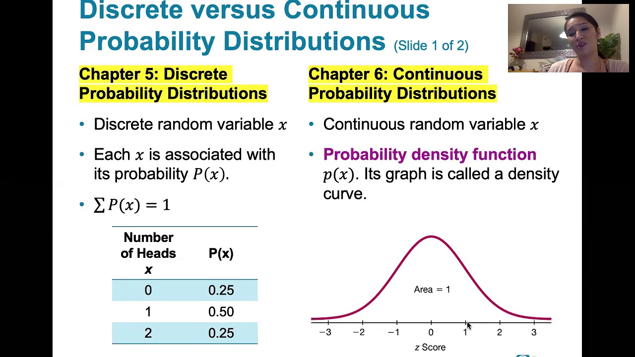
- 📈 The probability density function (PDF) describes the shape of a probability distribution
- 📊 For a continuous distribution, the total area under the curve is 1
- 🖊️ The CDF for a uniform distribution calculates the area to the left of some value X
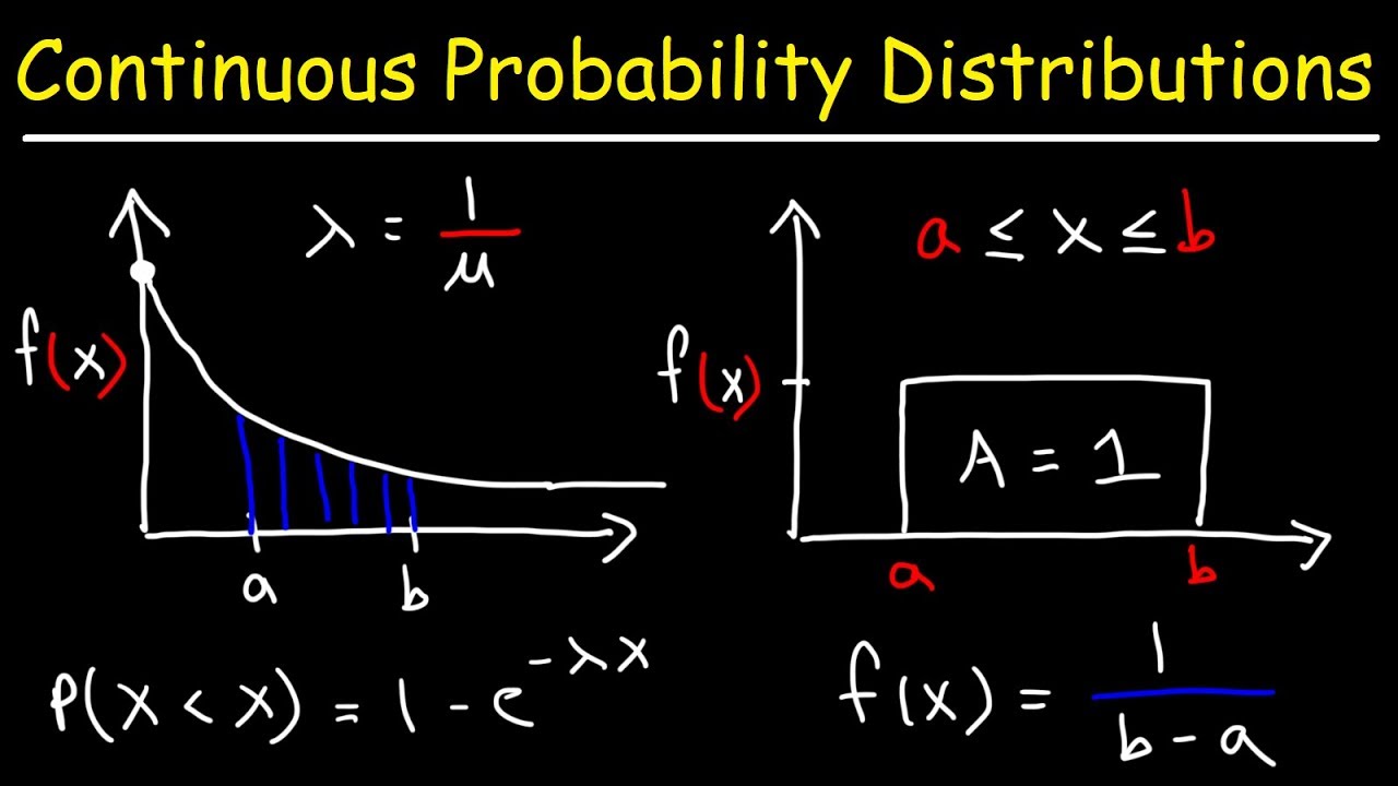
- ⛓ For an exponential distribution, the PDF is lambda * e^(-lambda * X)
- 🔢 The CDF for an exponential distribution calculates the area to the left of some value X
- 🔭 The CDF can calculate probabilities between two points by subtracting the area to the left
- ❇️ For continuous distributions, P(X = x) = 0. We need a range of values to calculate area and probability
- 📐 The PDF describes the shape of the distribution (exponential, normal, uniform, etc.)
- 🎯 The key difference between the PDF and CDF is that the CDF calculates accumulated probability or area under the curve
Q & A
What is the difference between a probability density function (PDF) and a cumulative distribution function (CDF)?
-The PDF, denoted f(X), describes the shape of the probability distribution and gives the height of the curve at a point X. The CDF gives the area under the curve up to a point, which represents the accumulated probability.
What is the formula for the CDF of a uniform distribution?
-The CDF for a uniform distribution is given by F(X) = (X - a) / (b - a), which calculates the area of a rectangle with base X - a and height 1 / (b - a).
What does the parameter lambda represent for an exponential distribution?
-Lambda is the rate parameter for an exponential distribution. It is equal to 1/mean. Lambda also represents the y-intercept and maximum value of the exponential distribution.
What is the formula for the PDF of an exponential distribution?
-The PDF of an exponential distribution is f(X) = lambda * exp(-lambda * X), where lambda is the rate parameter.
How can you use the CDF to find the probability between two values a and b?
-You can subtract the CDF values at the endpoints, i.e. F(b) - F(a). This gives the area under the curve between a and b.
Why is the probability 0 that X takes on an exact value for continuous distributions?
-Since continuous distributions are defined along an interval and have no width at a single point, the probability is 0 that X takes on an exact value.
What does the total area under a probability distribution curve represent?
-The total area under any probability distribution curve sums to 1, representing total probability.
What is the range of values for a CDF?
-The CDF ranges from 0 to 1, since it represents accumulated probability.
Can you calculate the area to the right using the CDF?
-Yes, you can subtract the CDF value from 1 to obtain the area to the right of that point, since the total area sums to 1.
How are probability density functions calculated for discrete distributions?
-For discrete distributions, the probability density function gives the probability mass at each individual, discrete value rather than over a continuous interval.
Outlines
📈 Defining PDFs and CDFs
This paragraph defines probability density functions (PDFs) and cumulative distribution functions (CDFs). It explains that PDFs describe the shape of a distribution, while CDFs calculate the accumulated probability or area under the distribution curve up to a certain point. Examples of PDFs and CDFs for uniform and exponential distributions are provided.
📉 Using CDFs to Calculate Areas
This paragraph explains how to use CDFs to calculate area under a distribution curve. It shows how to find the area to the left or right of a point, as well as the area between two points, for an exponential distribution. Key concepts covered include using CDFs to find probabilities of X less than or equal to some value.
📊 Key Points and Review
The last paragraph summarizes key learnings. It emphasizes that PDFs define distribution shape while CDFs calculate accumulated probability up to a point. It also notes that for continuous distributions, the probability X equals exactly some value is 0, while the probability over an interval of X values can be greater than 0.
Mindmap
Keywords
💡cumulative distribution function
💡probability density function
💡uniform distribution
💡exponential distribution
💡continuous distribution
💡area under the curve
💡rate parameter
💡probability density
💡interval probability
💡accumulated probability
Highlights
The cumulative distribution function calculates the area under the curve up to some point of interest.
The probability density function describes the shape of a distribution; the CDF gives the area under the curve.
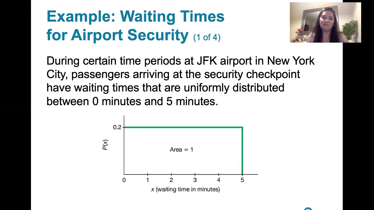
For a uniform distribution, the PDF is a constant between two endpoints.
The CDF for a uniform distribution calculates the area to the left of some value X.
For an exponential distribution, the PDF defines the curve's shape and height at point X.
The CDF for an exponential distribution gives the area under the curve to the left of X.
The area under an exponential curve to the right of X is e^(-λx).
Use the CDF to find the probability X lies between two values by subtracting areas.
The probability of X equaling one exact value is 0 for continuous distributions.
The PDF describes a distribution's shape; the CDF gives accumulated probability.
For continuous distributions, P(a ≤ X ≤ b) = P(a < X < b).
The probability density function f(X) defines a distribution's shape.
The cumulative distribution function calculates accumulated probability.
Use the CDF to find probability between two values by subtracting areas under the curve.
The probability X equals one exact value is 0 for continuous distributions.
Transcripts
Browse More Related Video
Continuous Probability Distributions - Basic Introduction

Probability Distribution Functions (PMF, PDF, CDF)

Elementary Stats Lesson #12
6.1.2 The Standard Normal Distribution - Uniform Distributions
Lecture 14: Location, Scale, and LOTUS | Statistics 110
6.1.1 The Standard Normal Distribution - Discrete and Continuous Probability Distributions
5.0 / 5 (0 votes)
Thanks for rating: