AP Calculus BC Lesson 7.5
TLDRThis video lesson introduces Euler's method for approximating solutions to differential equations, using a specific example where the differential equation is dy/dx = x - y/2. The process is illustrated step-by-step, showing how to approximate the value of f(2) given the initial condition f(1) = 3. The method involves creating a slope field, plotting the initial condition, and then following the slope field to estimate the solution curve. The video also explains how to use tangent lines at the initial condition and at subsequent points to improve the approximation. The concept is further applied to multiple scenarios, including those with different step sizes and initial conditions, demonstrating the method's flexibility and application in solving differential equations.
Takeaways
- 📚 Euler's method is a technique used to approximate solutions to differential equations given an initial condition.
- 🔍 The initial condition is a specific point on the solution curve of the differential equation.
- 🌐 The slope field of a differential equation visually represents the slopes (dy/dx) at various points in the Cartesian plane.
- 📈 To approximate a solution, one starts at the initial condition and follows the flow of the slope field.
- 🔜 Euler's method involves creating tangent lines at points on the solution curve to approximate the value of the function at other points.
- 🛣️ The tangent line's equation is derived using the point-slope form (y - y1 = m(x - x1)), where m is the slope (dy/dx) at a given point.
- 📊 The accuracy of Euler's method increases with the number of steps or the smaller the step size.
- 📌 The method can be applied to find approximate values of the function at specific x-coordinates by iteratively finding slopes and constructing tangent lines.
- 📐 When using Euler's method, it's important to remember that the results are approximations and may not be perfectly accurate.
- 📝 In practice, one can use a table of values or a differential equation to find the derivative (dy/dx) at a point.
- 🔄 Euler's method can be used to approximate values for functions defined by integrals or other mathematical expressions, not just differential equations.
Q & A
What is Euler's method used for in the context of this lesson?
-Euler's method is used to approximate solutions to differential equations when given an initial condition.
What is an initial condition in the context of differential equations?
-An initial condition is a point that lies on the solution curve of a differential equation.
How does the slope field represent the differential equation dy/dx = x - y/2?
-The slope field visually represents the possible slopes of the solution curves at various points in the xy-plane, which helps in sketching the solution curves.
How can the value of f(2) be approximated if f(1) = 3?
-By sketching the solution curve using the slope field and finding the tangent line at the initial condition (1, 3), the value of f(2) can be approximated by following the tangent line to the x-coordinate of 2.
What is the point-slope form of a line and how is it used in Euler's method?
-The point-slope form of a line is y - y1 = m(x - x1), where m is the slope, (x1, y1) is a known point on the line, and (x, y) are the coordinates of a point on the line. In Euler's method, it is used to find the equation of the tangent line at a given point, which helps in approximating the solution curve.
Why is the approximation of f(2) using the tangent line not perfect?
-The approximation is not perfect because the tangent line is an approximation itself, and as we move further away from the point of tangency, the reliability and accuracy of the approximation decrease.
How does the step size affect the accuracy of Euler's method?
-The smaller the step size, the more accurate the approximation tends to be, as the tangent line is more frequently updated to match the local slope of the solution curve, resulting in a closer approximation to the actual solution.
What is the process of approximating the value of f(3) using Euler's method?
-After approximating f(2), the process involves finding the slope at the approximated point (2, f(2)) using the differential equation, creating a new tangent line with this slope, and then using it to approximate the value of f(3).
How does the AP style example differ from the previous examples?
-The AP style example specifies the use of Euler's method with a certain number of equal-sized steps, whereas the previous examples involved creating tangent lines based on the local slope at each point without specifying the number of steps or their size.
What is the significance of the table in the multiple-choice question involving f'(x)?
-The table provides the values of f'(x), which are the derivatives of f(x), at selected x-values. This information is used in place of the differential equation to find the slopes for the tangent lines in Euler's method.
How does the problem involving f(x) as an integral use Euler's method?
-In the problem where f(x) is defined as an integral, the method involves finding the derivative f'(x) to approximate the slopes for the tangent lines, and then using Euler's method to approximate the value of f(3) starting from x=1 with a step size of 1.
What is the process for finding the value of K in the problem involving f(x) = ∫(1 to x) -3t^2 dt with initial condition f(1) = 2K?
-The process involves finding the derivative f'(x) = -3x^2, using Euler's method to approximate f(2) with the given step size, and then solving the resulting equation 5 = 8K for K.
Outlines
📚 Introduction to Euler's Method
This paragraph introduces Euler's method, a technique used to approximate solutions to differential equations given an initial condition. It presents an example involving a slope field for the differential equation dy/dx = x - y/2. The goal is to approximate the value of f(2) when f(1) = 3. The explanation includes breaking down the problem, sketching solution curves, and using tangent lines to approximate the solution's value at a specific point.
📈 Approximating f(3) with Tangent Lines
The paragraph continues the discussion on approximating the value of f(3) using tangent lines. It explains the process of constructing new tangent line segments based on the current slope and point, and how to use these to approximate the solution's value at subsequent x-coordinates. The example provided walks through the steps of finding the slope at x=2, constructing a new tangent line, and approximating f(3) using the updated slope. The paragraph emphasizes the iterative nature of Euler's method and the importance of using the most recent slope information for more accurate approximations.
🔍 Euler's Method with Equal Steps
This section delves into the application of Euler's method with equal-sized steps. It explains how to use the method to approximate the value of f(4) given a differential equation and an initial condition. The process involves finding the slope at the initial condition, constructing a tangent line, and using it to approximate the solution at the next step. The paragraph also introduces the concept of step size and how it affects the accuracy of the approximation, with smaller step sizes leading to more precise results.
📊 Euler's Method with Given Derivatives
The paragraph discusses a variation of Euler's method where the derivative of the function, f'(x), is provided in a table. It outlines the process of using the given f'(x) values to find the slope of the tangent line at specific x-values and then using these to approximate the function's value at the next step. The example given involves using the table to find the slope at x=3 and x=3.5 to approximate f(4). The paragraph highlights the utility of such tables in streamlining the approximation process.
🧮 Solving for Constants in Differential Equations
This paragraph presents a unique application of Euler's method where the goal is to solve for a constant, K, in a differential equation rather than approximating a function value. It explains how to use the given initial condition and the approximated value of the function at a later point to set up an equation and solve for the unknown constant. The example demonstrates the process of finding the derivative, using Euler's method to approximate the function value, and then solving for K using the given approximation of f(2) = 5.
📐 Euler's Method with Definite Integrals
The final paragraph discusses an Euler's method problem that involves the integral of a function from 1 to x. It explains how to find the derivative of the integral function, which serves as the slope for constructing the tangent line. The paragraph outlines the process of using Euler's method to approximate the value of the integral function at x=3, starting from x=1. It emphasizes the use of the fundamental theorem of calculus to simplify the integral and the importance of the step size in the approximation process.
Mindmap
Keywords
💡Euler's Method
💡Differential Equation
💡Initial Condition
💡Slope Field
💡Tangent Line
💡Point-Slope Form
💡Approximation
💡Step Size
💡Derivative
💡Solution Curve
💡Graphical Analysis
Highlights
Introduction to Euler's method for approximating solutions to differential equations.
Explanation of initial conditions and their role in solving differential equations.
Use of a slope field to visualize the differential equation dy/dx = x - y/2.
Graphical approximation of the solution curve by plotting the initial condition (1,3).
Approximation of f(2) using the tangent line method and the slope field.
Derivation of the tangent line equation using point-slope form and the differential equation.
Approximation of f(3) by changing the slope of the tangent line to match the current slope at x=2.
Discussion on the limitations of approximation as distance from the point of tangency increases.
Introduction to AP style problems and their structure for solving differential equations.
Euler's method applied to a different differential equation with a given initial condition f(1) = 2.
Use of two equal-length steps in Euler's method to approximate f(2) from x=1.
Demonstration of finding the slope at a given point using the differential equation.
Approximation of f(1.5) and f(3) using Euler's method and the derived tangent line equations.
Explanation of how the number of steps and step size affect the accuracy of Euler's method.
Application of Euler's method to a differential equation with a general form dy/dx = F'(x).
Use of a table of F'(x) values to approximate f(4) with a step size of 0.5 starting at x=3.
Solution of a non-traditional Euler's method problem involving the integral of a function.
Determination of the constant K in a differential equation using Euler's method and given approximations.
Final approximation of f(2) as 5 using a step size of 0.5 and starting at x=1.
Transcripts
Browse More Related Video

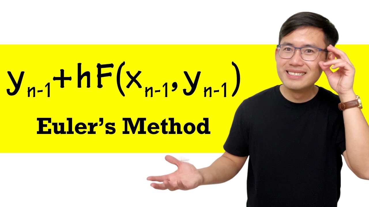
Euler's Method Differential Equations, Examples, Numerical Methods, Calculus
Calculus BC – 7.5 Approximating Solutions Using Euler’s Method
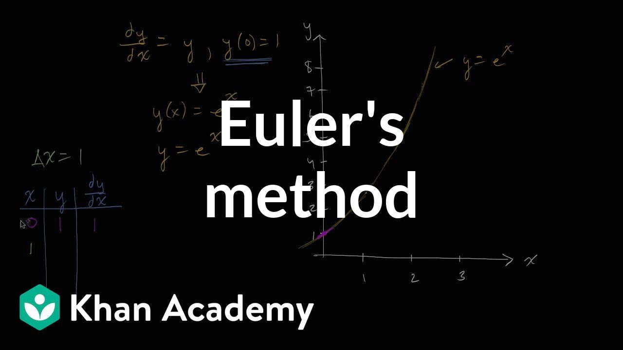
Euler's method | Differential equations| AP Calculus BC | Khan Academy

Euler's Method - Example 1
Euler's Method (introduction & example)
2008 AP Calculus AB Free Response #5
5.0 / 5 (0 votes)
Thanks for rating: