Probabilities from density curves | Random variables | AP Statistics | Khan Academy
TLDRThe video script explains how to calculate probabilities for continuous random variables using density curves. It first demonstrates finding the probability that a variable is less than four, using a simple rectangular distribution with equal probabilities. The area under the curve from one to four is calculated to determine a 75% chance. The second example involves a normal distribution of students' heights, where the script shows how to find the probability of a student being taller than 170 cm, using the empirical rule of the 68% area within one standard deviation from the mean. The probability of a height greater than 170 cm is approximately 16%, highlighting the use of Z-tables for precise values.
Takeaways
- 📊 The script discusses the concept of a density curve for continuous random variables, emphasizing the area under the curve represents probability.
- 🔢 The first example involves a uniform distribution where the random variable can take values from 1 to 5 with equal probability.
- 📉 The probability that the random variable x is less than four is calculated by finding the area under the density curve from 1 to 4, which is 0.75 or 75%.
- 📚 The second example involves a normal distribution of middle school students' heights with a mean of 150 cm and a standard deviation of 20 cm.
- 👦 The probability that a randomly selected student's height is greater than 170 cm is explored using the normal distribution.
- 📏 The mean of 150 cm and one standard deviation above the mean (170 cm) are used to visualize the problem on the density curve.
- 📉 The area under the normal distribution curve to the left of 170 cm is approximately 84%, derived from the empirical rule of normal distribution.
- 🔍 The probability of a height greater than 170 cm is found by subtracting the area to the left of 170 cm from 1, yielding approximately 0.16 or 16%.
- 📝 The use of a Z-table is suggested for a more precise calculation of probabilities in normal distributions.
- 🧮 The empirical rule is highlighted, stating that about 68.2% of data falls within one standard deviation of the mean in a normal distribution.
- 📈 The script illustrates the process of calculating probabilities using both a uniform and a normal distribution, emphasizing the importance of the area under the density curve.
Q & A
What is the range of values that the continuous random variable in the first example can take?
-The continuous random variable can take on values from one to five.
What is the probability distribution of the random variable in the first example?
-The probability distribution is uniform, meaning it has an equal probability of taking on any value from one to five.
How is the probability that x is less than four calculated in the first example?
-The probability is calculated by finding the area under the density curve from one to four, which is a rectangle with a height of 0.25 and a width of three, resulting in an area of 0.75 or 75%.
What is the significance of the entire area under the density curve being equal to one?
-The entire area under the density curve being equal to one represents the total probability of all possible outcomes, ensuring that the sum of probabilities for a continuous random variable is 100%.
What does the second example involve in terms of the distribution of middle school students' heights?
-The second example involves a normal distribution with a mean of 150 centimeters and a standard deviation of 20 centimeters for the heights of middle school students.
What is the mean height of the middle school students in the second example?
-The mean height of the middle school students is 150 centimeters.
How is the probability that a randomly selected student's height is greater than 170 centimeters found?
-The probability is found by calculating the area under the normal distribution curve to the right of 170 centimeters, which is done by subtracting the area below 170 from the total area of one.
What is the approximate area between one standard deviation below and above the mean in a normal distribution?
-The approximate area between one standard deviation below and above the mean in a normal distribution is about 68%.
How can the probability of a student's height being greater than 170 centimeters be estimated without a Z-table?
-The probability can be estimated by knowing that the area from the mean to one standard deviation above is approximately 34%, and then subtracting this from 50% to get the area above 170 centimeters, which is about 16%.
What is the general rule for the distribution of areas in a normal distribution around the mean?
-The general rule, known as the empirical rule or 68-95-99.7 rule, states that approximately 68% of the data falls within one standard deviation of the mean, 95% within two standard deviations, and 99.7% within three standard deviations.
Why might one use a Z-table to find a more precise probability in the second example?
-A Z-table provides the exact area under the standard normal curve to the left of a given Z-score, allowing for a more precise calculation of probabilities in normal distributions.
Outlines
📊 Understanding Probability Distributions
The script introduces the concept of a density curve for a continuous random variable, which can take values from one to five with equal probability. It explains how to calculate the probability that the variable x is less than four by finding the area under the curve from one to four. The area is calculated as 0.25 times three, resulting in a 0.75 or 75% probability. The script then moves on to discuss a more complex example involving the heights of middle school students, which are normally distributed with a mean of 150 cm and a standard deviation of 20 cm.
📚 Calculating Heights with Normal Distribution
This part of the script focuses on finding the probability that a randomly selected student's height is greater than 170 cm, given the normal distribution of the students' heights. It describes the process of visualizing the density curve, identifying the mean and standard deviation, and calculating the area under the curve that represents the desired probability. The script uses the empirical rule of normal distribution, stating that about 68% of the data falls within one standard deviation of the mean, to estimate that the area from the mean to 170 cm is approximately 34%. Subtracting this from the total area under the curve, which is 100%, gives an estimated probability of about 16% that a student's height is greater than 170 cm. For a more precise calculation, the script suggests using a Z-table.
Mindmap
Keywords
💡Density Curve
💡Continuous Random Variable
💡Probability Distribution
💡Area Under the Curve
💡Normal Distribution
💡Mean
💡Standard Deviation
💡Z-Table
💡Empirical Rule
💡Probability
💡Percentile
Highlights
The density curve describes the probability distribution for a continuous random variable that can take values from 1 to 5.
The random variable has an equal probability of taking any value from 1 to 5.
The area under the entire density curve represents a total probability of 1.
To find the probability that x is less than 4, calculate the area from 1 to 4 under the density curve.
The probability of x being less than 1 is zero, as shown by the density curve.
The area from 1 to 4 is a rectangle with height 0.25 and width 3, resulting in an area of 0.75.
The probability that x is less than 4 is 0.75 or 75%.
A set of middle school students' heights are normally distributed with a mean of 150 cm and standard deviation of 20 cm.
The probability that a randomly selected student's height is greater than 170 cm needs to be found.
The mean height of 150 cm and one standard deviation above (170 cm) are key points on the normal distribution curve.
The area between one standard deviation below and above the mean is approximately 68%.
The area from the mean to one standard deviation above the mean is about 34%.
The area below the mean in a normal distribution is 50%.
The combined area below 170 cm is approximately 84%.
The area above 170 cm, representing the probability of the height being greater than 170 cm, is calculated by subtracting 84% from 100%, resulting in about 16%.
Using a Z-table can provide a more precise value for the area above one standard deviation above the mean.
The general rule for normal distributions is that about 68% of the data falls within one standard deviation of the mean.
Transcripts
Browse More Related Video

Elementary Stats Lesson #11
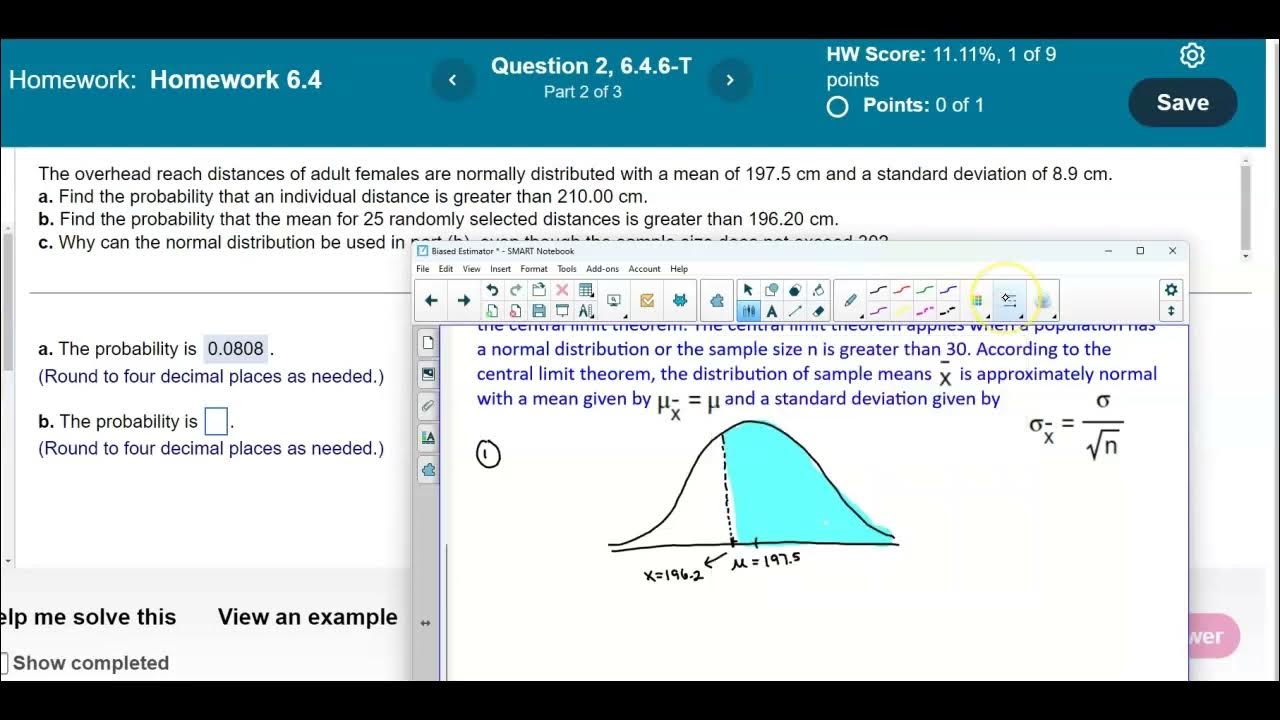
Math 14 HW 6.4.6-T Using the Central Limit Theorem
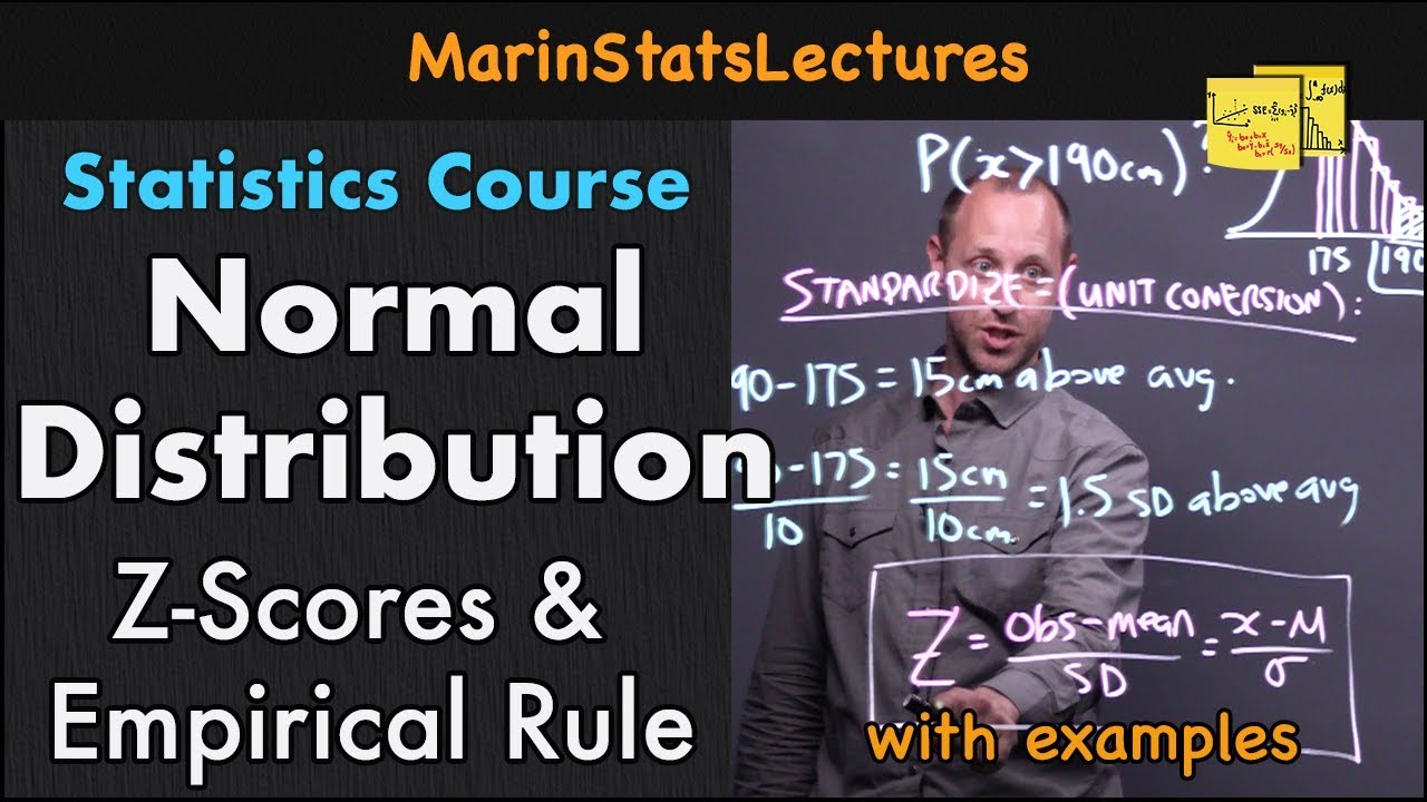
Normal Distribution, Z-Scores & Empirical Rule | Statistics Tutorial #3 | MarinStatsLectures

Normal Distribution, Z Scores, and Normal Probabilities in R | R Tutorial 3.3| MarinStatslectures
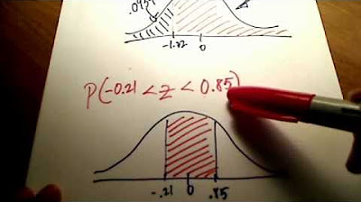
Stats: Finding Probability Using a Normal Distribution Table
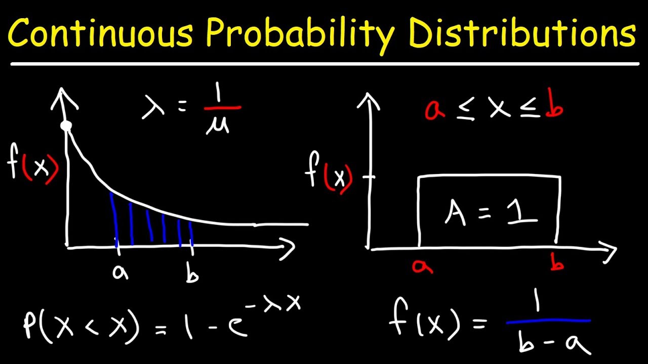
Continuous Probability Distributions - Basic Introduction
5.0 / 5 (0 votes)
Thanks for rating: