Normal Distribution, Z Scores, and Normal Probabilities in R | R Tutorial 3.3| MarinStatslectures
TLDRIn this instructional video, Mike Marin explains how to calculate probabilities, percentiles, and take random samples from a normally distributed variable. Using R's pnorm function, he demonstrates calculating probabilities for a variable with a mean of 75 and a standard deviation of 5. He also explains how to find quantiles with the qnorm function and plot the probability density function using the dnorm function. Additionally, he shows how to generate a random sample from a normal distribution with the rnorm command, noting that sample histograms may not always appear normal.
Takeaways
- 📚 The video is an educational tutorial focused on calculating probabilities, percentiles, and sampling from a normally distributed variable.
- 🔢 The example variable X is normally distributed with a mean of 75 and a standard deviation of 5.
- 📉 The pnorm command is used to calculate probabilities for a normal distribution, including lower and upper tail probabilities.
- 📈 The pnorm function can also be applied to calculate probabilities for a standard normal distribution (Z-scores).
- 📊 The qnorm function is utilized to determine quantiles or percentiles for a normal random variable, such as the first quartile.
- 📝 The dnorm function is used to plot the probability density function of a normal variable, showing the distribution's shape.
- 📈 A sequence of X values is created to demonstrate the probability density function over a range of values.
- 📊 The plot of the probability density function can be enhanced with a line connecting the points for a clearer visual representation.
- 📊 Adding a vertical line at the mean can provide a visual reference point on the probability density function plot.
- 🔄 The rnorm command is used to draw a random sample from a normally distributed population, as demonstrated with a sample size of 40.
- 🗂 Even though a sample is taken from a normally distributed population, the sample's histogram may not always appear normal.
Q & A
What is the main topic of the video by Mike Marin?
-The main topic of the video is calculating probabilities, percentiles, and taking random samples from a normally distributed variable.
What is the variable X in the example used in the video?
-Variable X is a normally distributed variable with a mean of 75 and a standard deviation of 5.
How can we calculate probabilities for a normal distribution in the video?
-Probabilities for a normal distribution can be calculated using the pnorm command in R.
What is the probability that X is less than or equal to 70 in the example?
-To calculate this, you would use the pnorm command with a mean of 75, a standard deviation of 5, and set the lower tail to true.
How do you calculate the probability that X is greater than or equal to 85?
-Use the pnorm command with a value of 85, a mean of 75, a standard deviation of 5, and set the lower tail to false for an upper tail probability.
What is the pnorm command used for in the context of a standard normal distribution?
-The pnorm command can be used to calculate probabilities for a standard normal distribution (Z-distribution) with a mean of 0 and a standard deviation of 1.
What is the Q Norm function used for?
-The Q Norm function is used to calculate quantiles or percentiles for a normal random variable.
How can you find the first quartile (25th percentile) of the variable X?
-Use the Q Norm function with the parameters for the mean, standard deviation, and set the lower tail to true to find the 25th percentile.
What is the purpose of the dnorm function in the video?
-The dnorm function is used to plot the probability density function for a normal variable.
How can you add a vertical line at the mean in a plot using R?
-In R, you can add a vertical line at the mean using the abline function with the 'v' argument set to the mean value, in this case, 75.
What command is used to draw a random sample from a normally distributed population in R?
-The rnorm command is used to draw a random sample from a normally distributed population with specified mean and standard deviation.
Why might a sample histogram from a normally distributed population not look normal?
-A sample histogram may not look normal due to the small sample size, which can lead to variability in the appearance of the distribution.
Outlines
📊 Calculating Probabilities and Percentiles for a Normal Distribution
In this segment, Mike Marin introduces the concept of calculating probabilities, percentiles, and taking random samples from a normally distributed variable. The example variable X is normally distributed with a mean of 75 and a standard deviation of 5. The pnorm command is used to calculate probabilities, such as the likelihood of X being less than or equal to 70, or greater than or equal to 85. The command's parameters, including the mean, standard deviation, and tail type (lower or upper), are explained. Additionally, the pnorm function is applied to calculate probabilities for a standard normal distribution (Z), and the qnorm function is introduced to determine quantiles or percentiles, such as the first quartile for X. The segment also covers plotting the probability density function using the dnorm function, with a demonstration of creating a sequence of X values, calculating densities, and plotting them. The process includes plotting a line to connect the points and adding a vertical line at the mean for clarity.
📈 Plotting and Sampling from a Normal Distribution
This paragraph discusses further analysis of a normal distribution, including plotting and sampling. The speaker provides a method to enhance the plot with titles, labels, and a vertical line at the mean using the abline function. The focus then shifts to drawing a random sample from a normally distributed population using the rnorm command, with parameters set for a mean of 75 and a standard deviation of 5, and a sample size of 40 observations. The resulting random sample is saved in an object named 'rand', and a histogram is presented to illustrate the distribution of the sample. It is noted that even though the sample comes from a normal distribution, the sample histogram may not appear perfectly normal, highlighting the variability inherent in sampling.
Mindmap
Keywords
💡Normal Distribution
💡Probability
💡Percentiles
💡pnorm Command
💡Z-Score
💡Quantiles
💡Probability Density Function (PDF)
💡dnorm Function
💡Histogram
💡Random Sample
💡Mean
💡Standard Deviation
Highlights
Introduction to calculating probabilities, percentiles, and random samples from a normally distributed variable.
Example used throughout the video: variable X with a mean of 75 and a standard deviation of 5.
Demonstration of calculating probabilities using the `pnorm` command in R.
Explanation of the lower tail and upper tail probabilities with examples.
Calculation of the probability that X is less than or equal to 70.
Calculation of the probability that X is greater than or equal to 85.
Use of the `pnorm` command to calculate probabilities for the standard normal distribution (Z).
Calculation of the probability that Z is greater than or equal to 1.
Introduction to the `qnorm` function for calculating quantiles or percentiles.
Calculation of the first quartile (25th percentile) for the variable X.
Creation of a plot of the probability density function using the `dnorm` function.
Step-by-step demonstration of plotting the probability density function for a normally distributed variable.
Adding a title and labels to the plot, and including a vertical line at the mean (75) using `abline`.
Drawing a random sample from a normally distributed population using the `rnorm` command.
Visualization of a histogram for the random sample drawn, with a note on the potential appearance of the sample histogram.
Transcripts
Browse More Related Video
Poisson Distribution in R | R Tutorial 3.2 | MarinStatsLectures
Probabilities from density curves | Random variables | AP Statistics | Khan Academy

Binomial Distribution in R | R Tutorial 3.1| MarinStatsLectures
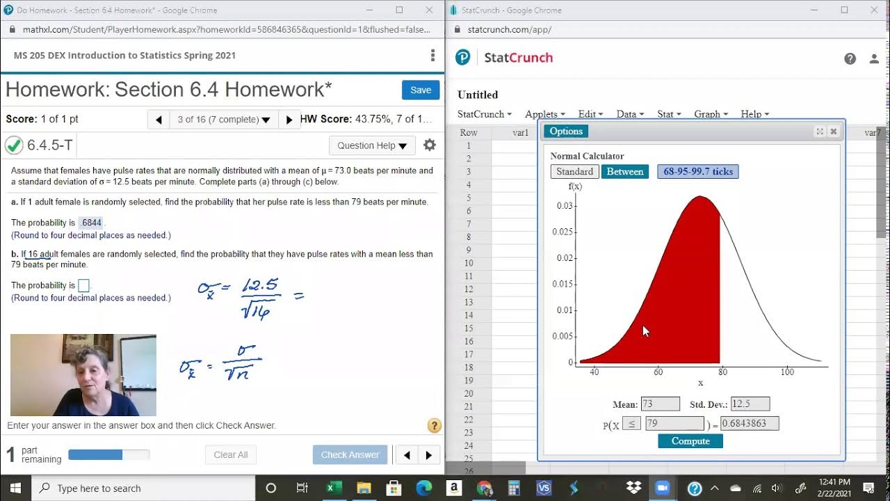
Calculating Probabilities of Sample Distributions with StatCrunch
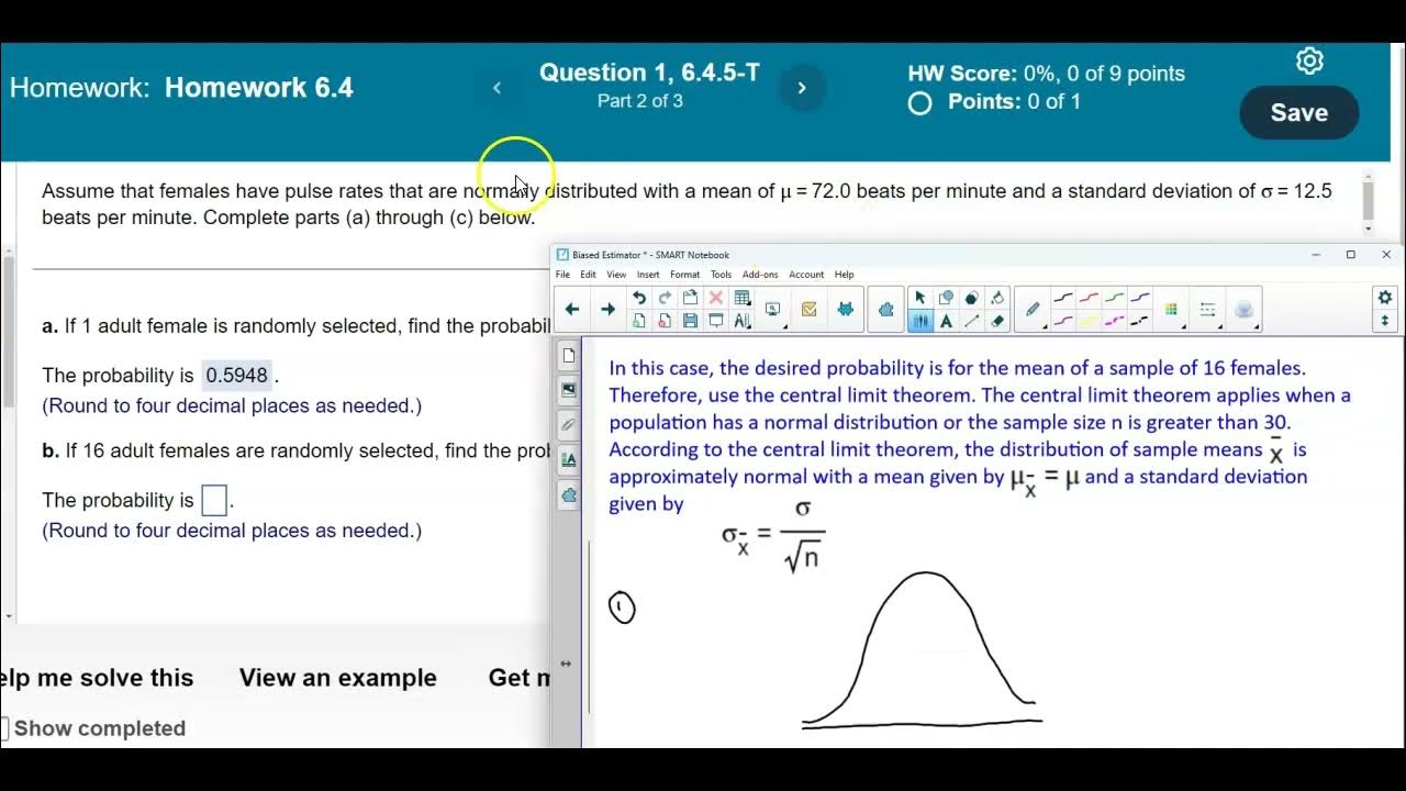
Math 14 HW 6.4.5-T Using the Central Limit Theorem

Working with Variables and Data in R | R Tutorial 1.8 | MarinStatslectures
5.0 / 5 (0 votes)
Thanks for rating: