Math 14 HW 6.4.6-T Using the Central Limit Theorem
TLDRThe script presents a statistical analysis involving normally distributed data with a mean of 197.5 cm and a standard deviation of 8.9 cm. It explains how to calculate the probability of an individual's distance exceeding 210 cm using the z-score method and a normal distribution calculator. Part B discusses the application of the central limit theorem to find the probability that the mean of 25 randomly selected distances is greater than 196.20 cm. The process involves determining a new z-score for the sample mean and using it to find the desired probability with a calculator, concluding with the correct answer selection based on the normal distribution's applicability.
Takeaways
- 📊 The script discusses a statistical problem involving a normal distribution with a mean of 197.5 cm and a standard deviation of 8.9 cm.
- 🔍 Part A of the problem asks to find the probability that an individual's distance is greater than 210.00 cm.
- 📈 The solution involves drawing a bell curve, labeling the mean, and identifying the area to the right of 210 cm on the curve.
- ➗ The z-score is calculated using the formula \( \frac{x - \text{mean}}{\text{standard deviation}} \), resulting in a z-score of 1.40.
- 📝 Z-scores are rounded to two decimal places for standardization.
- 🔢 The probability of a z-score greater than or equal to 1.40 is found using a statistical tool like StatCrunch, yielding a probability of 0.0808.
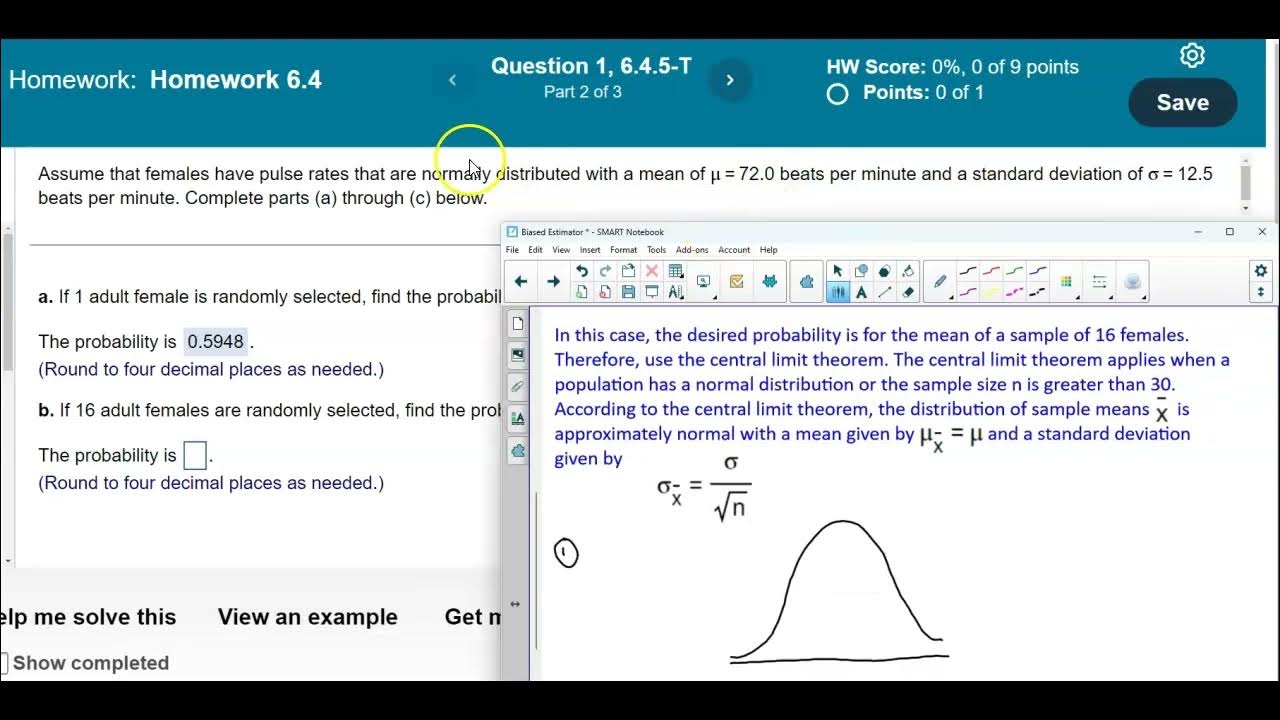
- 📚 Part B of the problem involves using the central limit theorem to find the probability that the mean of 25 randomly selected distances is greater than 196.20 cm.
- 📉 The central limit theorem states that the distribution of sample means is approximately normal, regardless of the population distribution, if the sample size is large enough (n > 30).
- 📐 The standard deviation of the sample means is calculated using the formula \( \frac{\text{population standard deviation}}{\sqrt{n}} \).
- 📉 A new z-score is calculated for the sample mean, resulting in -0.73 after rounding.
- 🔎 The probability of a z-score greater than or equal to -0.73 is determined to be 0.7673 using the statistical tool.
- 📌 The script emphasizes that the normal distribution can be used due to the original population's normal distribution, not because of the probability being less than 0.5 or other incorrect reasons mentioned.
Q & A
What is the mean height of the adult females in the given normally distributed population?
-The mean height of the adult females is 197.5 centimeters.
What is the standard deviation of the height of the adult females in the normally distributed population?
-The standard deviation of the height is 8.9 centimeters.
What is the probability that an individual's height is greater than 210 centimeters?
-The probability is calculated using the z-score, which in this case is 1.40, and the result is approximately 0.0808 or 8.08%.
How is the z-score calculated for an individual height of 210 centimeters?
-The z-score is calculated by subtracting the mean (197.5 cm) from the individual height (210 cm) and then dividing by the standard deviation (8.9 cm), which gives 1.40449, rounded to 1.40.
What is the significance of the z-score in the context of the script?
-The z-score standardizes the individual height measurement to the normal distribution, allowing us to find the probability of an event occurring beyond a certain value.
What statistical tool is used to determine the probability associated with the z-score?
-StatCrunch is used to determine the probability associated with the z-score.
What is the sample size considered in Part B of the script?
-The sample size considered in Part B is 25 randomly selected distances.
What is the probability that the mean of 25 randomly selected distances is greater than 196.20 centimeters?
-The probability is found using the z-score, which in this case is -0.73, and the result is approximately 0.7673 or 76.73%.
How does the Central Limit Theorem apply to the problem in Part B?
-The Central Limit Theorem is applied because the original population has a normal distribution, and the sample size (25) is large enough to use the theorem, which states that the distribution of sample means will be approximately normal.
What is the formula for the standard deviation of the sample means according to the Central Limit Theorem?
-The formula for the standard deviation of the sample means is the population standard deviation divided by the square root of the sample size (n).
Why is the normal distribution applicable in this scenario according to the script?
-The normal distribution is applicable because the original population is normally distributed, and the sample size is sufficient to invoke the Central Limit Theorem.
Outlines
📊 Calculating Probability with Z-Score
The first paragraph introduces a statistical problem involving the normal distribution of adult female heights with a mean of 197.5 cm and a standard deviation of 8.9 cm. The task is to find the probability that an individual's height is greater than 210 cm. The solution involves visualizing the data with a bell curve, identifying the mean and standard deviation, and calculating the z-score for 210 cm. The z-score is calculated as 1.40 after rounding, and the probability of this event is found using a statistical tool like StatCrunch, resulting in a probability of 0.0808.
📚 Applying the Central Limit Theorem
The second paragraph discusses the application of the Central Limit Theorem to find the probability that the mean of 25 randomly selected heights is greater than 196.20 cm. The theorem is applicable due to the original population's normal distribution or a sample size greater than 30. The solution involves calculating the standard deviation of the sample means using the formula (original standard deviation / √n), where n is the sample size. The z-score for the sample mean of 196.20 cm is calculated to be -0.73, and the probability of this event is determined using StatCrunch, yielding a result of 0.7673.
📉 Understanding the Conditions for Normal Distribution Use
The third paragraph addresses misconceptions about when the normal distribution can be used. It clarifies that the normal distribution is applicable because the original population is normally distributed, not because of the probability being less than 0.5, the finite population correction factor being small, or the mean being large. The correct answer is that the normal distribution is used due to the original population's normal distribution.
Mindmap
Keywords
💡Normal Distribution
💡Mean
💡Standard Deviation
💡Z-Score
💡Probability
💡Bell Curve
💡Central Limit Theorem
💡Sample Mean
💡StatCrunch
💡Finite Population Correction Factor
Highlights
The overhead reached distances of adult females are normally distributed with a mean of 197.5 centimeters and a standard deviation of 8.9 centimeters.
Part A requires finding the probability that an individual distance is greater than 210.00 centimeters using the population distribution.
A bell curve is drawn to visualize the problem, with the mean labeled at 197.5 centimeters.
The standard deviation is identified as 8.9 centimeters for the distribution.
The z-score formula is introduced to determine the probability of an individual's distance being greater than 210 centimeters.
The z-score is calculated as 1.40 after taking the difference between the individual value and the mean, divided by the standard deviation.
StatCrunch is used to find the probability associated with the z-score of 1.40, yielding a result of 0.0808.
Part B involves finding the probability that the mean of 25 randomly selected distances is greater than 196.20 centimeters.
The central limit theorem is applied to determine the distribution of sample means when the population is normally distributed.
A new bell curve is drawn to represent the distribution of sample means, with the mean set at 197.5 centimeters.
The standard deviation of the sample means is calculated using the formula involving the population standard deviation and the square root of the sample size.
The z-score for the sample mean is calculated as -0.73, indicating the deviation from the mean.
StatCrunch is utilized again to find the probability for the z-score of -0.73, resulting in a probability of 0.7673.
The normal distribution is chosen for calculations because the original population has a normal distribution, not because of other stated incorrect reasons.
The process demonstrates the application of the z-score and central limit theorem in statistical analysis.
The use of StatCrunch software is highlighted for calculating probabilities associated with z-scores.
The importance of understanding the distribution of individual values and sample means in statistical problems is emphasized.
Transcripts
Browse More Related Video
Math 14 HW 6.4.5-T Using the Central Limit Theorem

[6.4.6-T] Finding probabilities for different sample sizes using a nonstandard normal distribution
Normal Distribution, Z-Scores & Empirical Rule | Statistics Tutorial #3 | MarinStatsLectures

Math 14 HW 6.4.7-T Using the Central Limit Theorem
Probabilities from density curves | Random variables | AP Statistics | Khan Academy

Finding Probability of a Sampling Distribution of Means Example 1
5.0 / 5 (0 votes)
Thanks for rating: