Elementary Stats Lesson #11

walter dorman

27 Feb 202173:21

EducationalLearning

32 Likes 10 Comments

TLDRThis video script covers the transition from discrete to continuous random variables, focusing on the normal distribution. It introduces the concept of probability density functions (PDFs) and their properties, emphasizing the area under the curve as a key to understanding probabilities and proportions. The standard normal distribution, or z-distribution, is highlighted, and the script explains how to use z-tables and calculators to find areas under the curve, standardize data, and interpret z-scores. The empirical rule is discussed, along with practical examples involving SAT scores, to demonstrate the application of normal distribution in real-world scenarios.

Takeaways

📚 The lecture introduces Lesson 11, transitioning into the second half of the semester and focusing on Chapter 7, which discusses continuous random variables and normal distributions.
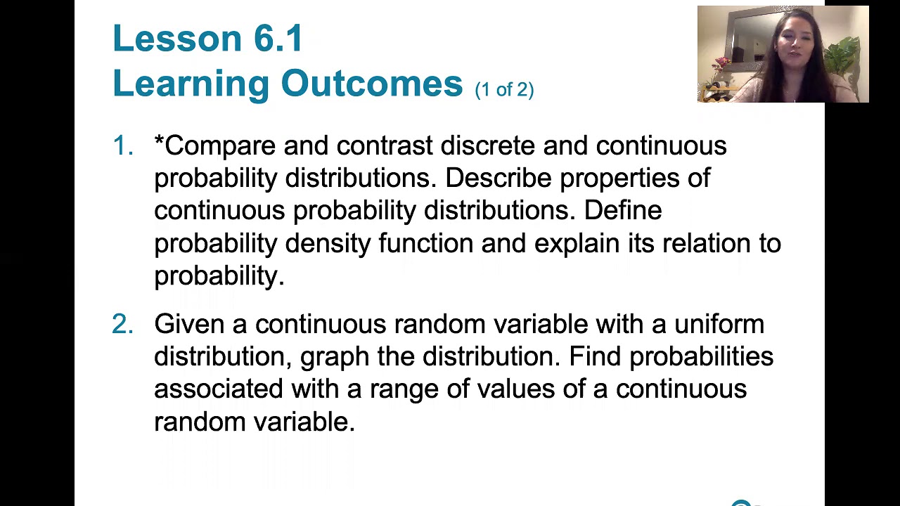
📈 Discrete random variables, covered in Chapter 6, are contrasted with continuous random variables, emphasizing the infinite number of possible outcomes in the latter.
🔍 The probability of a continuous random variable taking any exact value is zero due to the infinite number of possible outcomes, which is a fundamental concept in understanding continuous distributions.
📊 Normal distributions, or bell-shaped curves, are highlighted as an important type of continuous distribution, characterized by their symmetrical shape and specific properties.
📝 Key properties of probability density functions (pdfs) are discussed, including the fact that they are always above the x-axis and the area under the curve, which represents probabilities and proportions, equals one.
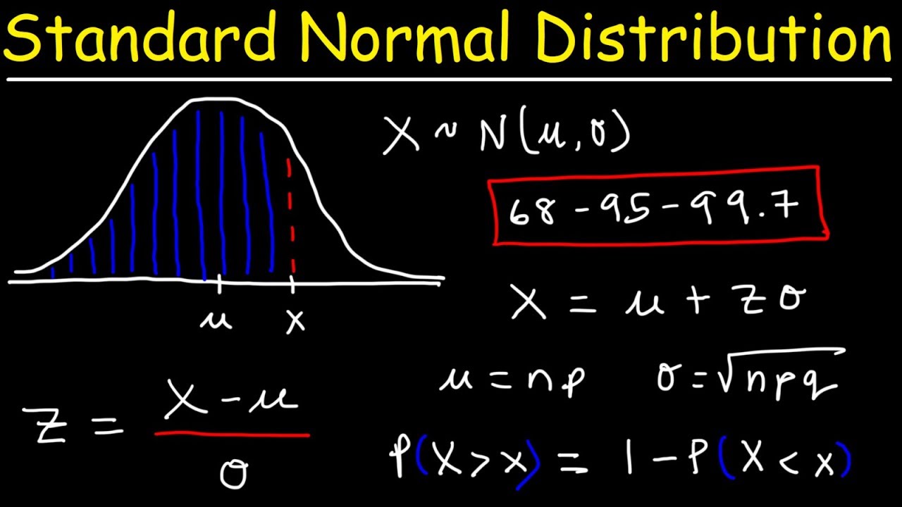
📐 The empirical rule is reiterated, stating that for a normal distribution, approximately 68%, 95%, and 99.7% of data fall within one, two, and three standard deviations from the mean, respectively.
📉 The concept of inflection points on a normal pdf is introduced, which are points where the curve changes concavity and can be used to estimate the standard deviation.
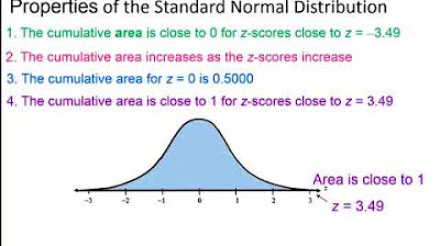
🌐 The standard normal distribution, with a mean of 0 and a standard deviation of 1, is explained as a basis for converting any normal distribution into z-scores for easier analysis.
🔢 Z-scores are used to standardize data and find areas under the normal curve, which represent probabilities or proportions, using either a z-table or a calculator for more precision.
📝 The z-table is detailed, explaining how to find left, right, and between areas under the curve, as well as how to invert the table to find z-scores given specific areas.
📊 The practical application of z-scores and the z-table is demonstrated with examples, including calculating percentiles and determining the proportion of a population within a certain range of scores.

Q & A

What is the main topic of the lesson in the transcript?
-The main topic of the lesson is the introduction to continuous random variables, specifically focusing on normal distributions and how to work with them, including the concept of probability density functions (PDFs) and z-scores.
What is a continuous random variable?
-A continuous random variable is a variable that can take on any value within an interval, as opposed to a discrete random variable which can only take on specific values. The set of possible values for a continuous variable is infinite.
Why is the probability that a continuous random variable equals any single particular value zero?
-The probability is zero because there are infinitely many possible values the variable can take on. The probability of any single specific outcome is the reciprocal of the number of possible outcomes, which is infinite in the case of continuous variables, thus resulting in a probability of zero.
What is a probability density function (PDF)?
-A probability density function is a function that describes the likelihood of a continuous random variable taking on a particular value. It is used to model the distribution of the variable and to calculate probabilities for ranges of values rather than specific values.
What are the key properties of a PDF?
-Two key properties of a PDF are: 1) it is always above the variable axis (x-axis), meaning it gives positive values, and 2) the area under the PDF between the function and the x-axis is always exactly equal to one, representing the total probability for all possible outcomes.
What is the empirical rule and how does it apply to normal distributions?
-The empirical rule states that for a normal distribution, approximately 68% of the data falls within one standard deviation of the mean, 95% falls within two standard deviations, and 99.7% falls within three standard deviations. It helps in understanding the spread of data around the mean in a normal distribution.
What is a standard normal distribution?
-A standard normal distribution, also known as the z-distribution, is a normal distribution with a mean of 0 and a standard deviation of 1. It serves as a baseline for normal distributions and allows for the standardization of different normal distributions for comparison and calculation purposes.
What are z-scores and how are they used in the context of normal distributions?
-Z-scores, or standard scores, are the values that represent how many standard deviations a data point is from the mean of a normal distribution. They are used to standardize different normal distributions so that they can be compared or analyzed using the same standard normal distribution curve.
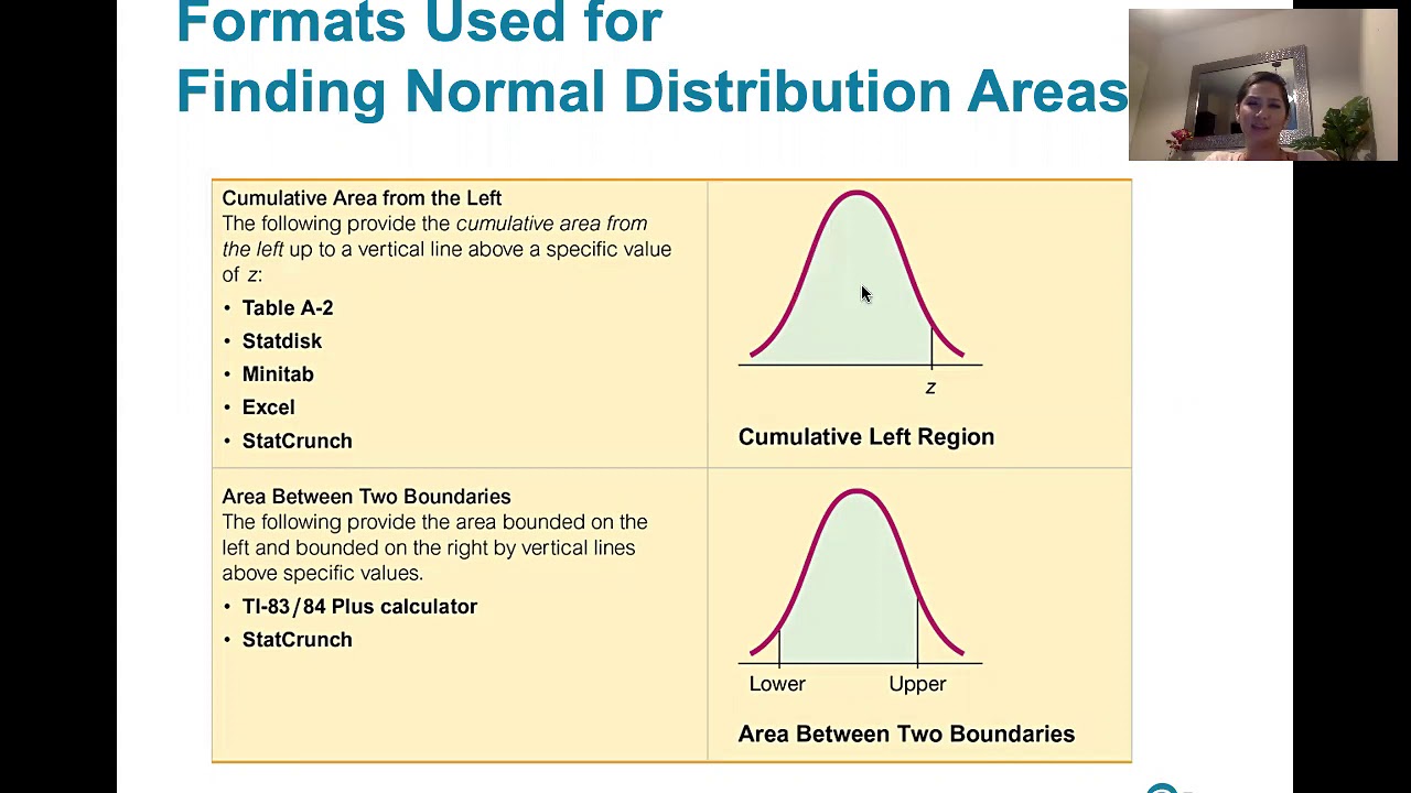
How can you find the area under a normal curve for a specific interval using a z-table?
-To find the area under a normal curve for a specific interval using a z-table, you first convert the original variable values into z-scores for the interval's endpoints. Then, look up the z-scores in the z-table to find the area to the left of each z-score. The area between the interval is found by subtracting the left area of the smaller z-score from the left area of the larger z-score.
What is the normal CDF program and how is it used to find areas under a normal curve?
-The normal CDF (Cumulative Distribution Function) program is a calculator function used to find the area under the standard normal curve between two given z-scores or values. It requires the input of the lower and upper bounds of the interval, the mean, and the standard deviation of the distribution. The program then calculates and returns the area, providing a precise probability for the specified interval.

Outlines

00:00

📚 Introduction to Continuous Random Variables

The instructor begins by welcoming students back and transitioning into the second half of the semester, focusing on Lesson 11 and Chapter 7 of the textbook. The main topic introduced is the concept of continuous random variables, contrasting them with discrete random variables covered in the previous lessons. A continuous random variable is characterized by an infinite number of possible outcomes, unlike the countable outcomes of discrete variables. The lesson aims to explore the complexities of continuous variables, starting with an example of the height distribution of men at a baseball game, which is symmetric and bell-shaped. The instructor poses a question about the probability of selecting a man exactly 71.1 inches tall, highlighting the fundamental difference in calculating probabilities for continuous variables compared to discrete ones.

05:02

📉 Understanding Probability Density Functions (PDFs)

The instructor delves into the concept of probability density functions (PDFs), which are used to model the distribution of continuous random variables. PDFs are mathematical models that provide a way to understand the distribution of data. The key properties of PDFs are discussed, emphasizing that the area under the curve between the variable axis and the PDF represents the total probability, which must equal one. The instructor also explains that the probability of a continuous variable taking any exact value is zero due to the infinite number of possible values. Instead, probabilities are calculated for intervals. The focus is on the normal distribution, a specific type of PDF that is symmetric and bell-shaped, and its importance in the chapter is highlighted.

10:02

📈 Key Properties of Normal Distributions

The instructor discusses the key properties of normal distributions, focusing on their symmetric bell shape and the importance of the mean, median, and mode being the same value in these distributions. The empirical rule is introduced, which states that for a normal distribution, approximately 68% of the data falls within one standard deviation of the mean, 95% within two standard deviations, and 99.7% within three standard deviations. The instructor also introduces the concept of inflection points on the normal curve, which are the points where the curve changes concavity and can be used to estimate the standard deviation.

15:03

📊 Analyzing a Histogram and Its Corresponding Normal Distribution

The instructor presents a data set of men's heights with corresponding classes, frequencies, and cumulative frequencies, leading to the construction of a histogram. The histogram is used to illustrate the distribution's shape, which is identified as symmetric and bell-shaped. The instructor then overlays a normal probability density function on the histogram to model the distribution, emphasizing the importance of the mean and standard deviation in characterizing a normal distribution. The process of transforming data into z-scores is introduced as a method for standardizing the data set to fit the standard normal model.

20:06

🔢 Standardizing Data and Using Z-Scores

The instructor explains the process of standardizing data by converting original variable values into z-scores, which are used to fit the data into the standard normal model. The formula for calculating z-scores is reviewed, and the instructor demonstrates how to convert a specific height into a z-score and vice versa. The purpose of standardizing data is to facilitate the calculation of areas under the normal curve, which correspond to probabilities.

25:07

📝 Using the Z-Table for Area Calculations

The instructor introduces the z-table, a tool for determining areas under the standard normal curve, which correspond to probabilities. The table is used to find the area to the left of a given z-score. The instructor demonstrates how to use the z-table to find left areas, right areas, and between areas, which are the probabilities of a z-score falling within a specified range. The importance of the z-table in calculating probabilities for normal distributions is emphasized.

30:08

🔍 Inverting the Z-Table to Find Z-Scores from Areas

The instructor shows how to use the z-table in reverse to find z-scores when given specific areas to the left or right of the z-score. This process involves finding the closest area in the table and identifying the corresponding z-score. The instructor provides examples of finding z-scores for areas to the left and areas to the right, highlighting the use of symmetry in the standard normal distribution.

35:09

🎯 Applying Z-Scores to SAT Scores and Percentiles

The instructor applies the concept of z-scores to SAT verbal test scores, which are approximately normally distributed. The mean and standard deviation of the SAT scores are provided, and the instructor demonstrates how to calculate z-scores for various SAT scores and interpret them as percentiles, showing the proportion of test takers with scores below a given SAT score.

40:10

📱 Utilizing Technology for Normal Distribution Calculations

The instructor introduces a calculator program called 'normal cdf' for calculating areas under the normal curve more precisely than the z-table. The program is used to find the percentage of students scoring between two SAT scores, providing a more accurate result than the table method. The instructor emphasizes the importance of this program for future calculations and assures that it will be extensively used and explained in the next lesson.

Mindmap

Keywords

💡Discrete Random Variable

A discrete random variable is a type of variable that can take on a countable number of distinct values, often used in probability experiments where outcomes can be counted. In the video, the concept is introduced as a foundation before moving on to continuous random variables, exemplified by the counting process in observing the results of a probability experiment.

💡Continuous Random Variable

This term refers to a variable that can take on any value within an interval, forming an infinite set of possible outcomes, unlike discrete variables. The video discusses the transition from discrete to continuous variables, highlighting the complexity of calculating probabilities for these types of variables, such as the height of men at a baseball game.

💡Normal Distribution

The normal distribution, also known as Gaussian distribution, is a probability distribution that is symmetric and bell-shaped. It is a fundamental concept in the video, where it is used to model continuous random variables such as the heights of men. The video explains that the normal distribution is characterized by its mean and standard deviation.

💡Probability Density Function (PDF)

A probability density function is a function that describes the likelihood of a continuous random variable taking on a particular value. In the video, PDFs are used to model the distribution of continuous variables, with the area under the PDF curve representing probabilities and proportions of the population within certain intervals.

💡Standard Deviation

The standard deviation is a measure of the amount of variation or dispersion in a set of values. In the context of the video, it is used to quantify the spread of the heights of men, with a smaller standard deviation indicating that the heights are closer to the mean value.

💡Mean

The mean, often referred to as the average, is the sum of all values in a data set divided by the number of values. In the video, the mean is used as a central value for the normal distribution of men's heights, indicating the average height.

💡Empirical Rule

The empirical rule is a statistical concept that states that for a normal distribution, about 68% of the data falls within one standard deviation of the mean, 95% within two, and 99.7% within three. The video uses the empirical rule to explain the distribution of men's heights around the mean.

💡Z-Score

A z-score is a standard score that indicates how many standard deviations an element is from the mean. In the video, z-scores are used to transform raw scores into a standard normal distribution, allowing for the use of the z-table to find areas under the normal curve and interpret data in a standardized way.

💡Z-Table

The z-table is a statistical tool used to find the area under the standard normal curve to the left of a given z-score. The video demonstrates how to use the z-table to determine probabilities and percentiles, which are essential for understanding the distribution of test scores like the SAT verbal test.

💡Normal CDF Program

The normal cumulative density function (CDF) program is a calculator tool that provides the area under the normal curve between two values, offering a more precise calculation than the z-table. The video introduces this program as a method to quickly find the probability that a continuous random variable falls within a specific range, such as the percentage of students scoring between certain SAT verbal scores.

Highlights

Introduction to the second half of the semester focusing on Lesson 11 and Chapter 7.

Transition from discrete random variables to continuous random variables.

Explanation of the concept of continuous random variables with infinite possible outcomes.

Introduction to normal distributions and the characteristics of continuous random variables.

Example of the height distribution of men at a baseball game as a normal distribution.

Discussion on the probability of a continuous random variable taking any single exact value being zero.

Explanation of probability density functions (pdfs) for modeling continuous distributions.

Properties of pdfs, including always being above the x-axis and the area under the curve equating to one.

The importance of the area under the pdf for determining probabilities and proportions within intervals.

Use of the empirical rule (68-95-99.7) for normal distributions to estimate proportions within standard deviations.

Identification of inflection points in normal pdfs to estimate standard deviation.

Notation for normal distributions using mean and standard deviation (x ~ N(μ, σ^2)).

Introduction to the standard normal distribution with mean 0 and standard deviation 1.

Process of standardizing data to z-scores for easier comparison and analysis.

Utilization of the z-table for finding areas under the standard normal curve.

Methods for calculating left, right, and between areas under the normal curve using the z-table.

Approach for finding z-scores associated with given areas using the z-table in reverse.

Application of normal distribution concepts to analyze SAT verbal test scores.

Calculation of percentiles and actual scores from z-scores using the standard normal distribution.

Introduction to the normal cdf calculator program for finding areas under the normal curve more precisely.

Conclusion emphasizing the importance of understanding normal distributions for future lessons.

Transcripts

Browse More Related Video

Elementary Statistics - Chapter 6 Normal Probability Distributions Part 1

Elementary Stats Lesson #12

Standard Normal Distribution Tables, Z Scores, Probability & Empirical Rule - Stats

Z-Scores, Standardization, and the Standard Normal Distribution (5.3)

6.1.0 The Standard Normal Distribution - Lesson Overview, Learning Outcomes

6.1.4 The Standard Normal Distribution - Given a range of z scores, find areas or probabilities.

Related Tags

Normal Distribution Probability Theory Discrete Variables Continuous Variables Educational Content Statistical Analysis Random Variables Symmetric Bell Curve Standard Deviation Z-Scores