Elementary Statistics - Chapter 6 Normal Probability Distributions Part 1

Joan DeRosa

8 Oct 201736:11

EducationalLearning

32 Likes 10 Comments

TLDRThis script introduces the concept of normal distributions, emphasizing its importance in statistics. It explains the bell-shaped curve, the significance of mean, median, and mode equality, and the curve's symmetry around the mean. The 68-95-99.7 rule is highlighted, explaining how data spreads around the mean in relation to standard deviations. The script also covers z-scores for data standardization, converting any normal distribution into a standard normal distribution with a mean of zero and a standard deviation of one. It concludes with practical examples of using calculators to find probabilities based on z-scores and normal distributions in real-world scenarios.

Takeaways

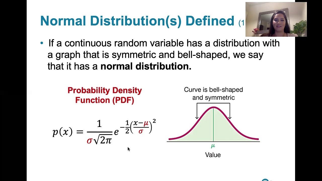
📊 The normal distribution is a continuous probability distribution characterized by a bell-shaped curve, which is fundamental in statistics.
📈 The properties of a normal distribution include its bell shape, and the equality of the mean, median, and mode, indicating a central tendency.
🔄 Normal distribution is symmetrical about the mean, dividing the curve into two equal halves, each representing 50% of the area under the curve.
🌐 The total area under the normal curve is equal to one, representing 100% probability, with the area signifying the likelihood of an event occurring.
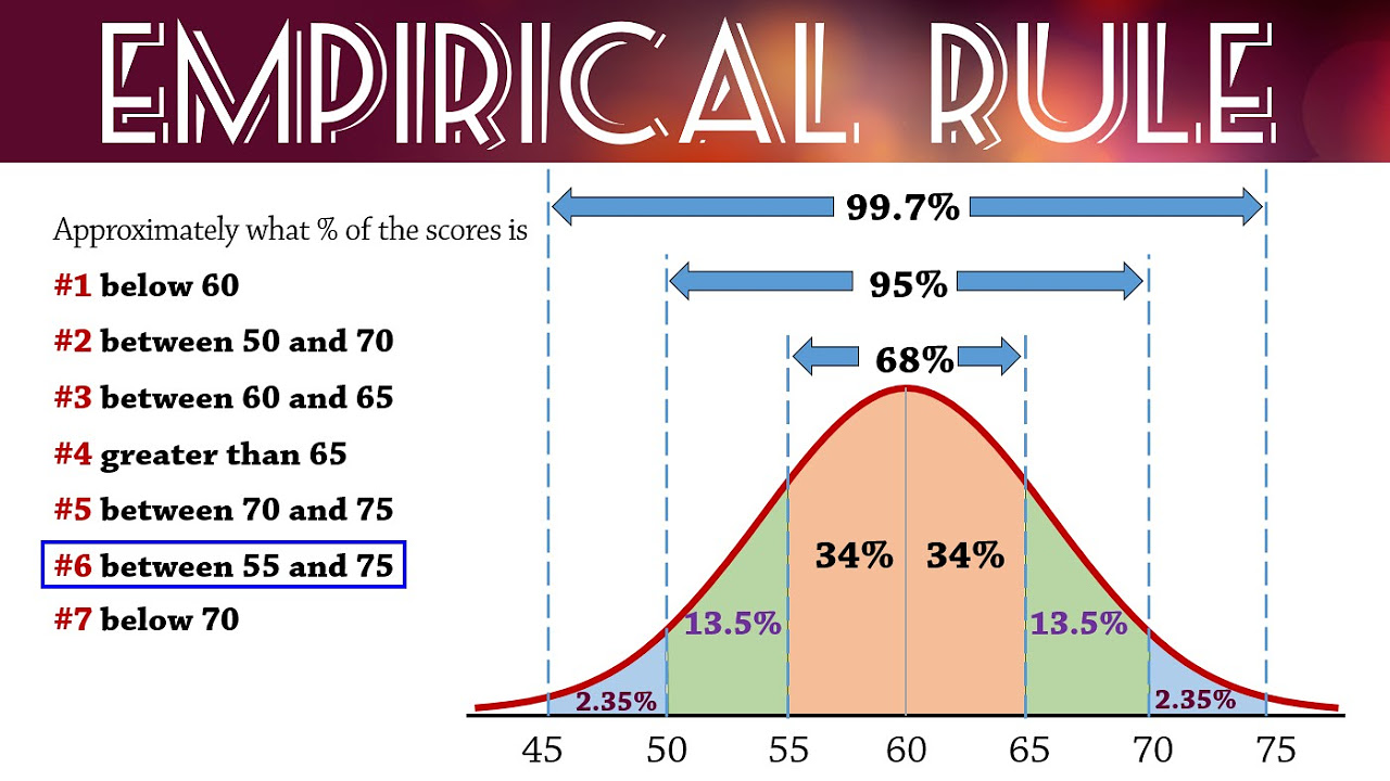
📉 The empirical rule (68-95-99.7 rule) states that about 68% of data falls within one standard deviation of the mean, 95% within two, and 99.7% within three.
📍 A normal distribution can have any mean and any positive standard deviation, affecting the curve's position and spread.
🔢 Z-scores are used to standardize scores in a normal distribution, allowing for comparison of data values across different scales.
📉 A standard normal distribution has a mean of zero and a standard deviation of one, simplifying the comparison of data sets.
🔍 The mean of a standard normal distribution is at the center of the curve, with positive and negative Z values representing areas to the right and left of the mean, respectively.
➗ The formula for converting a normal distribution to a Z-score is (X - mean) / standard deviation, aiding in the comparison of different data sets.
📚 The standard normal distribution table or calculators can be used to find the area under the curve for a given Z-score, which corresponds to the probability of an event.

Q & A

What is a normal distribution?
-A normal distribution is a continuous probability distribution for a random variable X, characterized by a bell-shaped curve known as the normal curve. It is the most important continuous probability distribution in statistics.
What are the properties of a normal distribution?
-A normal distribution has several properties: it is bell-shaped, symmetric about the mean, and the mean, median, and mode are all equal. The total area under the curve is equal to one, representing a 100% probability.
What is the significance of the mean in a normal distribution?
-The mean in a normal distribution is significant because it represents the center of symmetry for the curve, dividing the area under the curve into two equal parts, each with an area of 50%.
What is the empirical rule or 68-95-99.7 rule in the context of normal distribution?
-The empirical rule states that in a normal distribution, approximately 68% of the data lies within one standard deviation of the mean, 95% within two standard deviations, and 99.7% within three standard deviations.
What is a standard normal distribution?
-A standard normal distribution is a specific type of normal distribution with a mean of zero and a standard deviation of one. It is also known as the Z-distribution.
What is a Z-score and how is it used in normal distribution?
-A Z-score is a standardized score that represents the number of standard deviations a data point is from the mean. It is used to compare data values on different scales and to convert any normal distribution into a standard normal distribution for easier comparison.
How can you find the area under the normal curve for a given Z-score?
-The area under the normal curve for a given Z-score can be found using a standard normal table or a calculator. The area represents the probability associated with that Z-score.
What is the difference between the area to the left and the area to the right of a Z-score on the standard normal distribution curve?
-The area to the left of a Z-score represents the probability of the random variable being less than that Z-score, while the area to the right represents the probability of the random variable being greater than that Z-score. The sum of these two areas is always equal to 1 (or 100%).
How can you use a calculator to find the probability associated with a Z-score?
-You can use the normal distribution function on a calculator, such as the 'normalcdf' function, to find the probability associated with a Z-score. You input the lower and upper bounds, the mean, and the standard deviation, and the calculator will provide the cumulative area, which is the probability.
What is the significance of the standard deviation in the shape of a normal distribution curve?
-The standard deviation determines the spread of the data in a normal distribution. A higher standard deviation results in a wider curve, indicating greater variability in the data, while a smaller standard deviation results in a narrower curve, indicating less variability.

Outlines

00:00

📊 Introduction to Normal Distributions

The script introduces normal distributions as a fundamental concept in statistics, characterized by a bell-shaped curve. It emphasizes the normal curve's importance and its properties, such as the equivalence of mean, median, and mode, and its symmetry around the mean. The total area under the curve equals one, representing probabilities ranging from 0 to 1. The script also explains the 68-95-99.7 rule, which describes the distribution of data relative to the mean and standard deviations, and how the normal distribution can vary in terms of mean and standard deviation, affecting the curve's shape and spread.

05:01

📈 Understanding Z-Scores and Standard Normal Distribution

This paragraph delves into z-scores, which standardize data from normally distributed sets, facilitating comparison across different scales. A standard normal distribution, with a mean of zero and a standard deviation of one, is introduced as a reference for converting any normal distribution into this standard form. The script explains how to calculate z-scores and the significance of positive and negative z-values in relation to the mean. It also details how to interpret areas under the standard normal curve as probabilities, using a normal distribution table or calculator.

10:05

🔢 Using Calculators for Normal Distribution Probabilities

The script provides a tutorial on using calculators to find areas under the normal curve, which correspond to probabilities for given z-scores. It explains the process of entering data into the calculator, including how to represent negative infinity for areas to the left of a z-score and positive infinity for areas to the right. The importance of using the correct menu options and understanding the calculator's output in terms of probabilities is highlighted, with examples of how to interpret results in the context of the normal distribution.

15:08

📝 Calculating Areas and Probabilities with Z-Scores

This section explains how to calculate the area to the left or right of a z-score, and between two z-scores, using both standard normal tables and calculators. It clarifies the process of finding the area to the right by subtracting the area to the left from one, and emphasizes the importance of recognizing the direction of shading when using a calculator. The script also provides examples of how to input data into older and newer calculator models to find the desired probabilities.

20:10

🤔 Applying Normal Distribution in Real-World Scenarios

The script presents real-world applications of normal distribution, such as estimating the probability of cell phone users replacing their phones within a certain timeframe or shoppers spending a specific amount of time in a supermarket. It demonstrates how to convert given data into z-scores and use calculators to find the probability of an event occurring within a normal distribution, emphasizing the importance of understanding the mean, standard deviation, and the direction of shading in probability calculations.

25:11

🛒 Estimating Shopper Behavior Using Normal Distribution

This paragraph focuses on a marketing scenario where understanding shopper behavior in terms of time spent in a supermarket is valuable. The script uses the normal distribution to calculate the probability of shoppers staying in the store for varying lengths of time, given the average and standard deviation of their stay. It also shows how to estimate the number of shoppers expected to stay beyond a certain time threshold within a larger group, highlighting the practical use of normal distribution in predicting outcomes.

30:11

📉 Interpreting Normal Distribution for Probability Estimations

The final paragraph reinforces the concept of using normal distribution to estimate probabilities in various scenarios. It provides examples of how to calculate the probability of shoppers staying in a store for more than a given time and how to adjust calculations based on different intervals. The script stresses the importance of correctly identifying the direction of shading (left or right) and the use of calculators to find the area under the curve, which represents the probability of an event.

Mindmap

Keywords

💡Normal Distribution

Normal distribution, also known as Gaussian distribution, is a continuous probability distribution that is characterized by its bell-shaped curve. In the video, it is described as the most important continuous probability distribution in statistics. It is pivotal because it allows for the prediction and analysis of data points around a central mean. The script explains that the mean, median, and mode of a normal distribution are equal, indicating a symmetrical distribution where data points are most frequently found near the center.

💡Normal Curve

The normal curve is the graphical representation of a normal distribution. As depicted in the script, it is bell-shaped and symmetrical, with the mean at its center. The curve is significant in the video as it visually represents the distribution of data and the probabilities associated with different values. The total area under the normal curve equals one, which corresponds to a 100% probability of all possible outcomes in a normal distribution.

💡Empirical Rule (68-95-99.7 Rule)

The empirical rule is a set of probabilities that describe the distribution of data points within a normal distribution. As detailed in the script, it states that approximately 68% of data points fall within one standard deviation of the mean, 95% within two standard deviations, and 99.7% within three standard deviations. This rule is fundamental for understanding the spread of data and the likelihood of extreme values in a normal distribution.

💡Standard Deviation

Standard deviation is a measure of the amount of variation or dispersion in a set of values. In the context of the video, it is used to quantify the spread of data points around the mean in a normal distribution. A larger standard deviation indicates a greater spread of data, while a smaller standard deviation indicates that data points are closer to the mean. The script uses the standard deviation to explain the 68-95-99.7 rule and to calculate z-scores.

💡Z-Score

A z-score is a standard score that indicates how many standard deviations an element is from the mean. In the video, z-scores are used to standardize data values from a normal distribution, making it possible to compare data on different scales. The script explains the process of converting a raw score into a z-score and how z-scores facilitate the comparison of data across various normal distributions.

💡Standard Normal Distribution

A standard normal distribution is a specific type of normal distribution with a mean of zero and a standard deviation of one. The video script introduces the concept to demonstrate how any normal distribution can be converted into this standard form for easier comparison and analysis. The standard normal distribution is also known as the Z-distribution and is used to find probabilities associated with z-scores.

💡Line of Symmetry

In the context of the normal distribution, the line of symmetry refers to the vertical line that passes through the mean and divides the normal curve into two equal halves. As mentioned in the script, this line is crucial because it implies that the area to the left and right of the mean is equal, each constituting 50% of the total area under the curve.

💡Cumulative Area

The cumulative area under the normal curve to the left or right of a specific z-score represents the probability of the random variable falling within a certain range. The script explains how the cumulative area increases as the z-score increases, and it is used to find probabilities for various ranges in a normal distribution. For example, the cumulative area close to zero for a z-score of -3.49 indicates a very low probability of occurrence.

💡Normalcdf (Normal Cumulative Distribution Function)

Normalcdf is a function used to calculate the area under the normal curve to the left of a given z-score. In the video script, it is used in calculators to find probabilities associated with z-scores. The function is essential for determining the likelihood of a random variable falling within a specified range in a normal distribution.

💡Scientific Notation

Scientific notation is a way of expressing very large or very small numbers and is used in the video script when dealing with probabilities that are close to zero. It involves representing a number as the product of a decimal between 1 and 10 and a power of 10. In the context of the video, scientific notation is used to express probabilities that are numerically very small, such as those associated with extreme z-scores.

💡Probability

Probability is a measure of the likelihood that a particular event will occur, and in the video, it is closely related to the area under the normal curve. The script explains that the area shaded under the normal curve represents the probability of a random variable falling within a certain range. For instance, the probability of a random variable being less than a certain value is found by calculating the area to the left of that value under the normal curve.

Highlights

Introduction to normal distributions, emphasizing the normal curve's importance in statistics.

Properties of normal distribution include a bell-shaped curve with equal mean, median, and mode.

Symmetry of the normal distribution curve around the mean, dividing the area into two equal parts.

Total area under the normal curve equals one, representing 100% probability.

The 68-95-99.7 rule, explaining the distribution of data within one, two, and three standard deviations from the mean.

Any normal distribution can have any mean and any positive standard deviation.

Z-scores standardize data values, allowing comparison across different scales.

Conversion of any normal distribution to a standard normal distribution for ease of comparison.

Standard normal distribution has a mean of zero and a standard deviation of one.

Z-scores are calculated using the formula (X - mean) / standard deviation.

Properties of a standard normal distribution, including the cumulative area close to zero for Z values far from the mean.

Using a normal distribution table or calculator to find areas and probabilities associated with Z values.

Guidelines for finding areas to the left, right, and between Z-scores using standard normal distribution.

Practical application of normal distribution in determining probabilities in real-world scenarios, such as cell phone usage.

Calculating the probability of shoppers spending different amounts of time in a supermarket using normal distribution.

Estimating the number of shoppers expected to stay in a store beyond a certain time using normal distribution probabilities.

The importance of understanding the direction of shading (left or right) when finding areas under the normal curve.

The significance of the mean in determining the area under the normal curve for values on either side of it.

Transcripts

Browse More Related Video

6.1.3 The Standard Normal Distribution - Normal Dist. and Properties of the Standard Normal Dist.

The Normal Distribution and the 68-95-99.7 Rule (5.2)

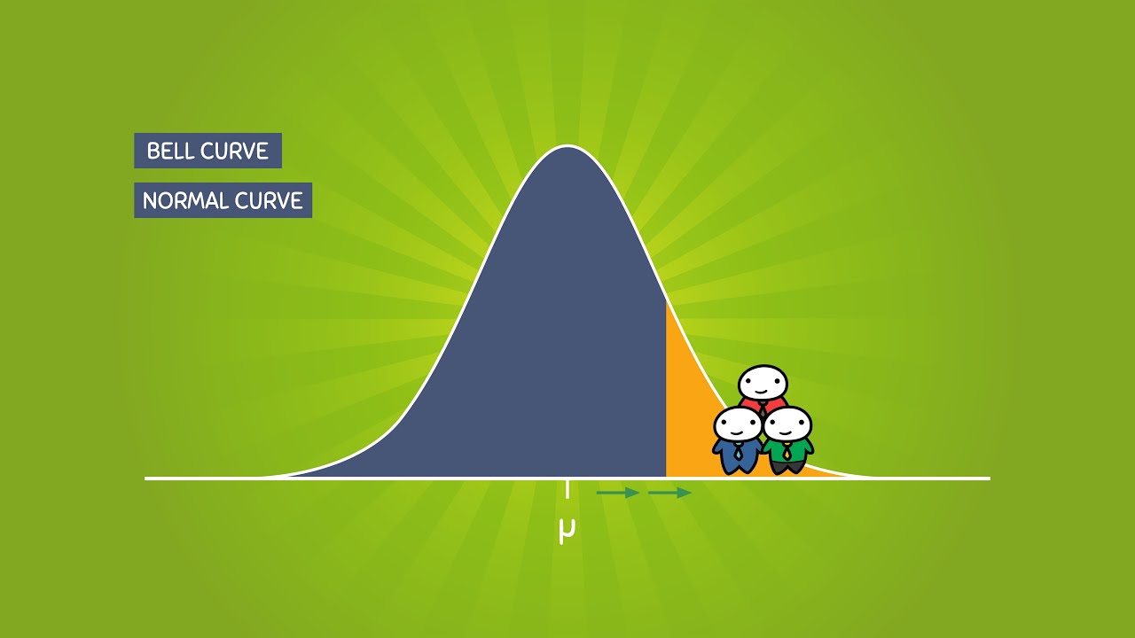
What is a Bell Curve or Normal Curve Explained?

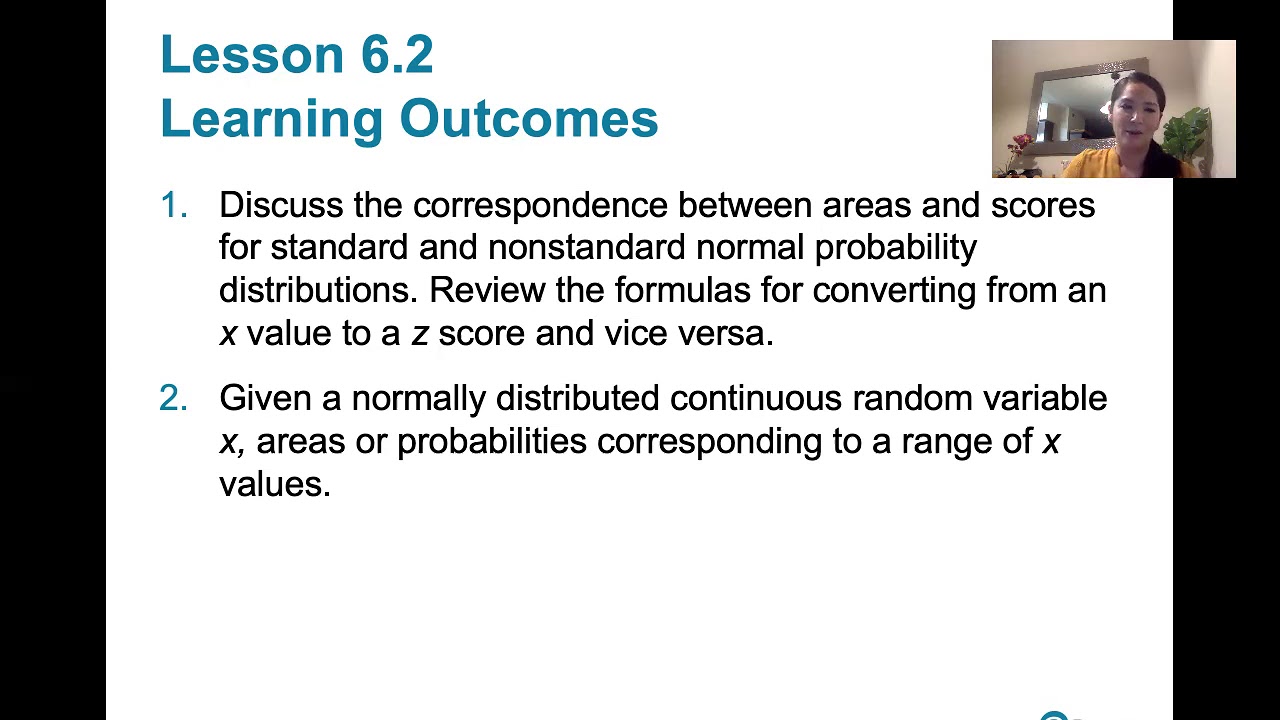
6.2.0 Nonstandard Normal Distributions - Lesson Overview, Learning Outcomes, Key Concepts

Normal Distribution & Probability Problems

Empirical Rule (68-95-99.7) for Normal Distributions

Related Tags

Normal Distribution Statistics Probability Bell Curve Mean Median Mode Empirical Rule Standard Deviation Z-Score Data Analysis Statistical Inference