Elementary Stats Lesson #12
TLDRThis transcript outlines a statistics lesson focusing on continuous random variables, particularly those with a normal distribution. The lesson explains the use of probability density functions (PDFs) and the importance of the area under the normal curve for probability and proportion questions. Two primary methods for calculating these areas are discussed: using a z-table and a calculator with a normal cumulative distribution function (CDF). The transcript also covers the inverse normal function for finding scores corresponding to specific percentiles and introduces the concept of normal probability plots for assessing the normality of a population, especially useful for small sample sizes.
Takeaways
- 📚 The lesson is part of a statistics course, focusing on the second half of chapter 7, which introduces continuous random variables and their distribution modeling using probability density functions (PDFs).
- 📉 For continuous random variables with a symmetric bell-shaped distribution, a normal model is appropriate, denoted as 'normal mu sigma', where 'mu' is the mean and 'sigma' is the standard deviation.
- 📊 The area under a normal curve is crucial for answering probability questions, representing either the proportion of the population within a certain interval or the probability of a random individual falling within that interval.
- 🔢 Two primary methods for finding areas under the normal curve are discussed: the 'table method' using a z-table for standardization of scores, and the 'technology method' using a calculator's normal cumulative distribution function (CDF).
- 🔍 The z-table method requires converting original values into z-scores by subtracting the mean and dividing by the standard deviation, then using the table to find the area.
- 🧮 The calculator method simplifies the process by directly computing the area under the normal curve for specified intervals without the need for manual standardization.
- 📝 Three types of area calculations are highlighted: left area, right area, and between area, each serving different probability questions regarding the distribution.
- 🤔 The script emphasizes the importance of understanding the process for calculating these areas, including using the z-table for direct and complement probabilities, and the calculator for more precise results.
- 📉 The video script provides examples using the reading speeds of sixth-grade students, demonstrating how to calculate probabilities of different reading speeds using both methods.
- 👀 The concept of 'unusual' events is introduced, defined as those with a probability less than 0.05, and methods for calculating such probabilities are discussed.
- 🔄 The script also covers how to find the value of x corresponding to a given area or percentile using both the z-table (inversely) and a calculator's inverse normal function.
- 📊 Lastly, the script touches on assessing normality, especially for small sample sizes, using a normal probability plot (NPP) to determine if the population distribution can be considered normal and thus if a normal model is appropriate.
Q & A
What is the main topic of the lesson in the transcript?
-The main topic of the lesson is dealing with continuous random variables, specifically those with a normal distribution, using probability density functions (PDFs) and z-tables for various calculations.
Why can't a table be used for a continuous random variable?
-A table is not sufficient for a continuous random variable because it is not discrete. Instead, a model, specifically a probability density function (PDF), is used to represent the distribution of the variable.
What is a normal PDF used for in statistics?
-A normal PDF is used to model the distribution of a continuous random variable that has a symmetric, bell-shaped distribution. It is represented with the notation 'normal mu sigma' where mu is the mean and sigma is the standard deviation.
How is the area under a normal curve interpreted in the context of the lesson?
-The area under a normal curve is interpreted in two ways: as a proportion of the population within a certain interval of values, and as the probability that a randomly selected individual falls within that interval.
What are the two methods for finding areas under the normal curve discussed in the transcript?
-The two methods discussed are the z-table method, which involves standardizing values and looking up probabilities in the z-table, and the technology method, which uses a calculator program to compute the exact area under the curve for a given interval.
What is a z-score and how is it calculated?
-A z-score is a standard score that indicates how many standard deviations an element is from the mean. It is calculated by subtracting the mean (mu) from the value (x) and then dividing by the standard deviation (sigma) of the set.
What is the purpose of the normalcdf program on a calculator?
-The normalcdf program on a calculator is used to compute the exact area under the normal curve between two values (a and b), which corresponds to the probability that a random individual falls within that interval.
How can you determine if a variable's distribution is approximately normal using a small sample size?
-For small sample sizes, a normal probability plot (NPP) is used to assess if the population distribution is approximately normal. The plot should show an approximately linear pattern if the distribution is normal.
What is the significance of the inverse normal program on a calculator?
-The inverse normal program (invNorm) on a calculator is used to find the value of x that corresponds to a specific percentile or area to the left, given the mean and standard deviation of the distribution.
What is the standard approach to determine if an event is considered unusual based on its probability?
-An event is considered unusual if its probability is less than 0.05, unless the problem specifies a different threshold. This is a common standard in statistics for identifying rare or unusual events.
Outlines
📚 Introduction to Continuous Random Variables
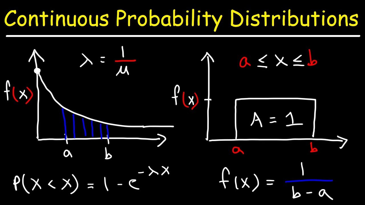
This paragraph introduces the concept of continuous random variables and the necessity of using a probability density function (pdf) instead of a table due to the variable's continuous nature. The focus is on the normal distribution, which is characterized by its symmetric bell shape and is denoted by the notation 'normal mu sigma'. The paragraph sets the stage for discussing the properties and applications of the normal distribution in statistical problems.
📈 Understanding the Normal Distribution and Area Calculations
The paragraph delves into the importance of the area under the normal curve for answering statistical questions. It explains two interpretations of this area: as a proportion of the population within a certain interval and as the probability of a randomly selected individual falling within that interval. The process of calculating these areas is discussed, emphasizing the use of a normal curve and the interval of interest, whether it's a left area, right area, or between area calculation.
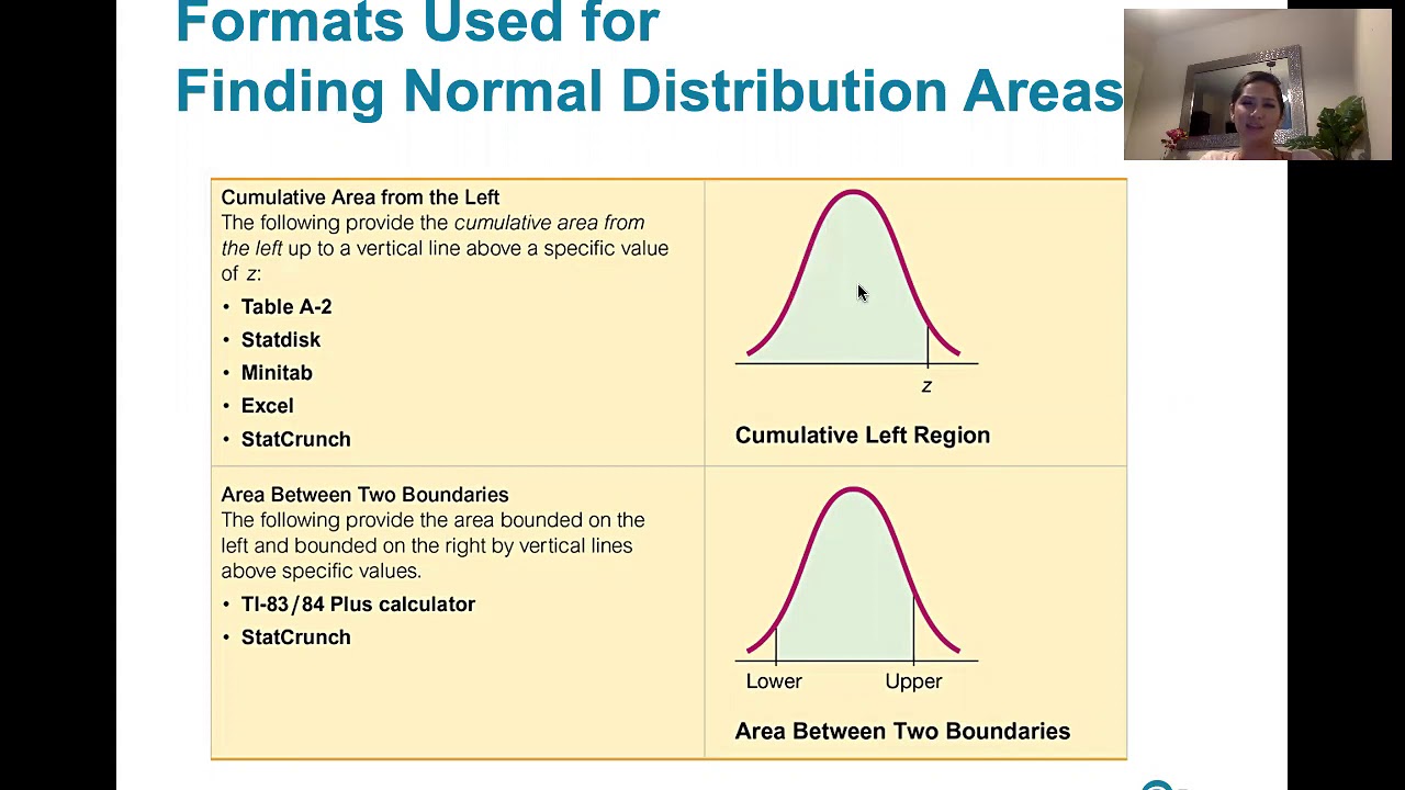
🔢 Methods for Calculating Areas Under the Normal Curve
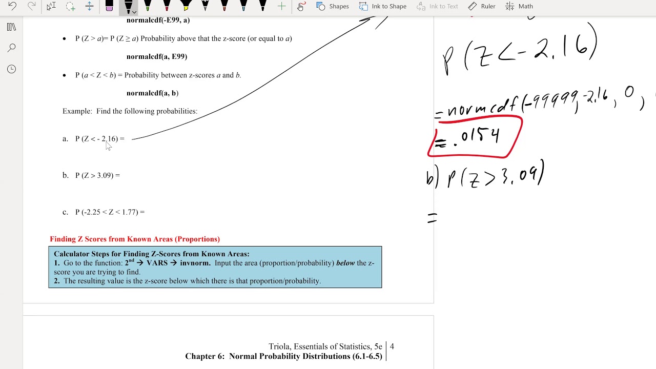
This section outlines two methods for calculating areas under the normal curve: the z-table method and the calculator method. The z-table method requires standardizing the variable into z-scores, while the calculator method uses a built-in program to compute the exact area. The paragraph provides general notes on using the z-table for different area calculations and the steps involved in each method.
🛠️ Calculator Techniques for Normal Distribution Problems
The paragraph discusses the use of calculator programs for finding left, right, and between areas under the normal curve. It explains how to input values for the mean, standard deviation, and bounds of interest to calculate probabilities. Tips are provided for using the calculator effectively, including how to input very large negative and positive numbers as boundaries.
📘 Examples of Applying Normal Distribution to Reading Speed Data
This paragraph presents an example using the normal distribution to analyze reading speeds of sixth-grade students. It demonstrates how to calculate the probability of a student reading at different speeds using both the z-table and calculator methods. The results from both methods are compared, showing a slight difference due to rounding in the z-table method.
🤔 Determining Unusual Reading Speeds Using Normal Distribution
The paragraph explores the concept of identifying unusual events by calculating the probability of a sixth-grade student reading at an unusually fast speed. It uses the normalcdf calculator program to determine that the probability of reading more than 200 words per minute is very low, indicating that such an event is indeed unusual.
🔍 Assessing Normality Through Normal Probability Plots
This section introduces the concept of assessing whether a population is normally distributed, especially when dealing with small sample sizes. It explains the use of normal probability plots (NPP) to determine if the data points fall approximately on a straight line, which would suggest normality. The paragraph also discusses the limitations of using histograms for small data sets and the industry standard for what constitutes a 'small sample'.
📊 Constructing and Interpreting Normal Probability Plots
The paragraph provides a step-by-step guide on how to construct a normal probability plot using a calculator and explains how to interpret the plot. It emphasizes the importance of looking for a linear pattern in the plot, which would indicate that the population is approximately normal. An example using the eruption times of Old Faithful Geyser is given to illustrate the process and the interpretation of the results.
🚀 Conclusion and Preview of Upcoming Statistical Inference Lessons
In the final paragraph, the instructor wraps up the lesson on normal distribution and its applications, highlighting the importance of understanding the material before moving on to the next chapters. The upcoming lessons are previewed, with a focus on statistical inference and how the tools introduced will be used to make determinations about populations based on sample data.
Mindmap
Keywords
💡Continuous Random Variable
💡Probability Density Function (PDF)
💡Normal Distribution
💡Z-Score
💡Z-Table
💡Normal CDF Program
💡Inverse Normal Program
💡Standard Deviation
💡Mean
💡Normal Probability Plot (NPP)
Highlights
Introduction to continuous random variables and the use of probability density functions (pdf) for their distribution.
Explanation of the normal distribution model for symmetric, bell-shaped continuous random variables, denoted as normal mu sigma.
Emphasis on the importance of the area under the normal curve for answering probability questions.
Two methods for calculating areas under the normal curve: the z-table method and the calculator method.
Detailed guide on using the z-table for left, right, and between area calculations.
Instructions on utilizing the normal cdf calculator program for exact area computations.
Process for determining unusual events based on the probability threshold of less than 0.05.
Example of calculating the probability of a sixth-grade student reading at an unusual speed.
Illustration of using both the z-table and calculator for probability calculations, highlighting the close results.
Introduction of the inverse normal distribution program for finding scores corresponding to specific percentiles.
Demonstration of how to use the inverse normal calculator for determining reading speeds at various percentiles.
Discussion on assessing normality of a population, especially important for small sample sizes.
Explanation of the normal probability plot (NPP) as a tool for assessing normality in small samples.
Procedure for constructing a normal probability plot on a calculator for small data sets.
Interpretation of the normal probability plot to determine if a population is approximately normal.
Real-world example using the times between eruptions of Old Faithful geyser to illustrate the NPP.
Final thoughts on the importance of population normality for statistical inference and upcoming lessons.
Transcripts
Browse More Related Video

5.0 / 5 (0 votes)
Thanks for rating: