Another simulation giving evidence that (n-1) gives us an unbiased estimate of variance
TLDRThe video script from Khan Academy user Justin presents a simulation that illustrates the rationale behind using n-1 as the divisor for calculating an unbiased estimate of population variance from a sample. The simulation uses a population with a uniform distribution from 0 to 100 and samples of size 50. It compares the results of calculating variance by dividing by n, n-1, and n-2. The findings show that dividing by n consistently underestimates the true variance, while dividing by n-1 provides a good estimate that converges to the actual population variance. Dividing by n-2, however, overestimates it. The video also visually represents the difference between using the sample mean and the population mean for variance calculation, highlighting that using the sample mean typically results in a lower variance estimate. The simulation concludes that dividing by n-1 is the appropriate method for obtaining an unbiased estimate of the population variance.
Takeaways
- 📊 The simulation by Justin from Khan Academy demonstrates the concept of calculating unbiased sample variance by dividing by n-1.
- 🔢 A population with a uniform distribution from 0 to 100 is used for the simulation, and samples of size 50 are taken from this population.
- 🧮 The sample variance is calculated three different ways: dividing by n, n-1, and n-2, to observe the impact on the estimate of the population variance.
- 🔍 As more samples are taken and variances are calculated, the mean of these variances is compared to the true population variance.
- 📉 Dividing by n consistently underestimates the true variance, even when averaging many sample variances.
- 🎯 Dividing by n-1 provides a good estimate, with the mean of the sample variances converging to the true variance.
- 📈 Dividing by n-2 results in an overestimation of the true variance, indicating it is not the correct approach.
- 📋 The simulation visually represents how the sample mean differs from the true mean and how this affects the calculation of variance.
- 📉 When using the sample mean to calculate variance (dividing by n), the calculated variance is always lower than if the population mean were used.
- 🔄 Dividing by n-1 sometimes underestimates and sometimes overestimates, but the mean of these variances converges to the true variance.
- 🤔 The shape of the graph when comparing the variance calculated with the sample mean versus the population mean is intriguing and invites further analysis.
- 📌 The entire graph of variances calculated with the sample mean sits below the horizontal axis, indicating a consistent underestimation when using the sample mean.
Q & A
What is the purpose of the simulation created by Justin?
-The simulation created by Justin is designed to provide an understanding of why dividing by n minus 1, rather than n, gives an unbiased estimate of the population variance when calculating the sample variance.
What type of distribution does the population in the simulation have?
-The population in the simulation has a uniform distribution, with a flat probabilistic distribution from 0 to 100.
What sample size is used in the simulation?
-The sample size used in the simulation is 50.
How does the simulation calculate variance for each sample?
-For each sample, the simulation calculates the sample variance by dividing by n, n minus 1, and n minus 2, and then takes the mean of these variances.
What happens when the sample variance is calculated by dividing by n?
-When the sample variance is calculated by dividing by n, the simulation shows that the true variance is underestimated, even when taking the mean of many sample variances.
What is observed when the sample variance is calculated by dividing by n minus 1?
-When the sample variance is calculated by dividing by n minus 1, the simulation indicates that a good estimate of the true variance is obtained, with the mean of the sample variances converging to the true variance.
What occurs when the sample variance is calculated by dividing by n minus 2?
-When the sample variance is calculated by dividing by n minus 2, the simulation demonstrates that the true variance is overestimated, with the mean of the sample variances being higher than the actual value.
How does the simulation visualize the comparison between the sample mean and the true mean?
-The simulation visualizes this comparison by plotting each sample on the horizontal axis, where the distance to the right indicates how much more the sample mean is than the true mean, and to the left indicates how much less.
What does the vertical axis represent in the simulation's visualization?
-The vertical axis in the simulation's visualization represents the difference between the variance calculated using the sample mean and the variance that would be calculated if the population mean was known.
What shape does the graph take when comparing the variances calculated with the sample mean versus the population mean?
-The graph takes an interesting shape that sits below the horizontal axis, indicating that the variance calculated with the sample mean is always lower than if the population mean was used.
What is the significance of the shape of the graph in the simulation?
-The shape of the graph is significant as it provides insight into the bias of the sample variance calculation. It prompts further thinking about why this shape occurs and what it implies about the estimation process.
What conclusion can be drawn from the simulation regarding the calculation of unbiased sample variance?
-The simulation concludes that using n minus 1 as the denominator when calculating the sample variance provides an unbiased estimate of the population variance, as evidenced by the convergence of the mean of the sample variances to the true variance.
Outlines
📊 Understanding Sample Variance Calculation
The first paragraph introduces a simulation by Khan Academy user Justin, aimed at explaining the rationale behind using 'n-1' in the formula for calculating an unbiased estimate of population variance from a sample. The simulation uses a population with a uniform distribution from 0 to 100 and takes samples of size 50. For each sample, the script describes calculating the sample variance by dividing by n, n-1, and n-2, and observing how the mean of these variances converges to the true variance of the population. The findings indicate that dividing by n consistently underestimates the true variance, while dividing by n-1 provides a good estimate, and dividing by n-2 overestimates it. The paragraph also introduces a visual representation comparing the sample mean to the population mean, highlighting the tendency to underestimate variance when using the sample mean for calculations.
Mindmap
Keywords
💡Unbiased estimate
💡Population variance
💡Sample variance
💡Sampling
💡Sample size (n)
💡Divisor (n, n-1, n-2)
💡Convergence
💡Simulation
💡Flat probabilistic distribution
💡Sample mean
💡Population mean
💡Underestimation and Overestimation
Highlights
The simulation demonstrates why dividing by n-1 provides an unbiased estimate of population variance when calculating sample variance.
A population with a uniform distribution from 0 to 100 is used for the simulation.
Samples of size 50 are taken from the population.
Sample variance is calculated by dividing by n, n-1, and n-2 for each sample.
Means of variances calculated in different ways are taken to observe convergence.
Dividing by n consistently underestimates the true variance.
Dividing by n-1 provides a good estimate converging to the true variance.
Dividing by n-2 results in an overestimation of the true variance.
The simulation visually compares sample mean variances to population mean variances.
Using the sample mean to calculate variance typically results in a lower variance than using the population mean.
Dividing by n-1 sometimes overestimates and sometimes underestimates, but the mean of these variances converges.
The graph of variances calculated with the sample mean always sits below the horizontal axis, indicating an underestimate.
The shape of the graph when comparing sample mean variances to population mean variances is interesting and worth further consideration.
The simulation provides a clear visual representation of the impact of using different denominators in variance calculation.
The simulation results support the rationale for using n-1 as the divisor for an unbiased estimate of variance.
The simulation is a practical application of statistical theory to demonstrate the concept of unbiased estimation.
The use of continuous sampling and averaging variances provides insight into the behavior of different variance calculation methods.
The simulation offers an innovative method for visualizing statistical concepts related to variance estimation.
Transcripts
Browse More Related Video
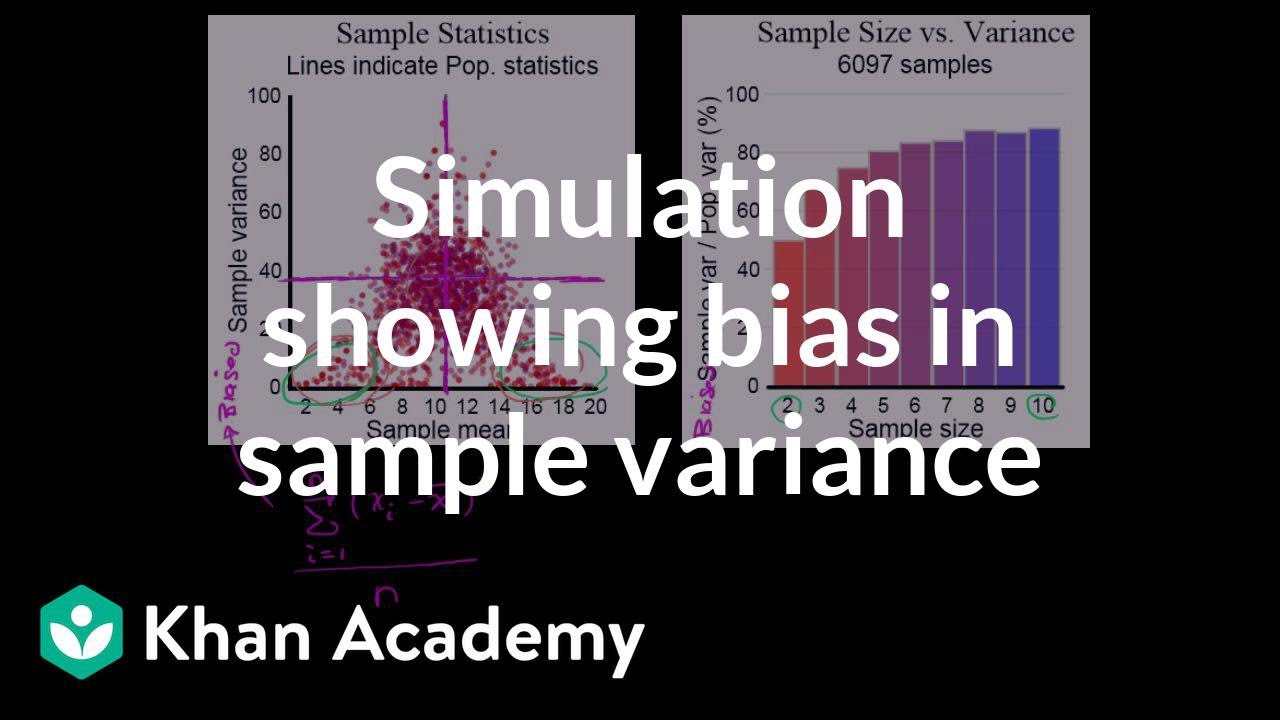
Simulation showing bias in sample variance | Probability and Statistics | Khan Academy
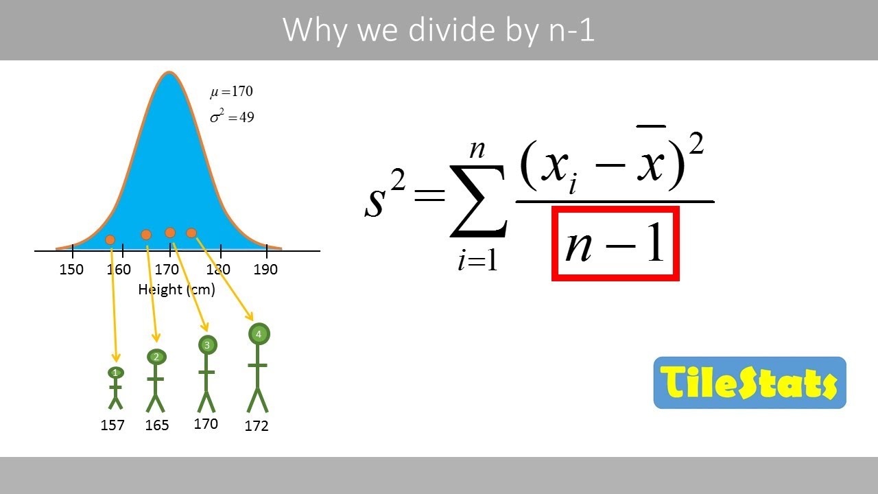
Why do we divide by n-1 and not n? | shown with a simple example | variance and sd
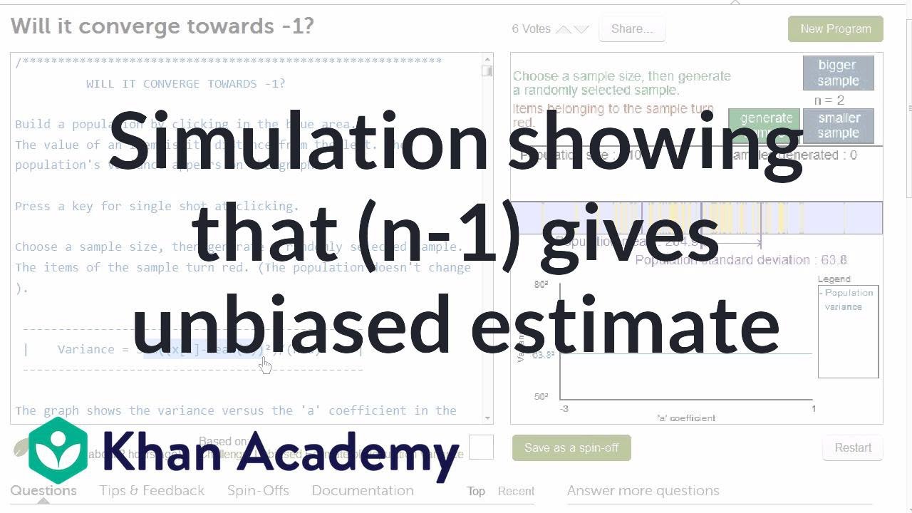
Simulation providing evidence that (n-1) gives us unbiased estimate | Khan Academy
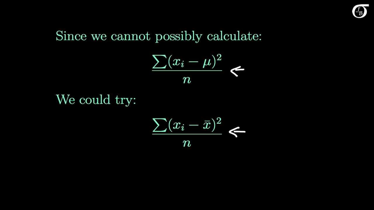
The Sample Variance: Why Divide by n-1?
Review and intuition why we divide by n-1 for the unbiased sample | Khan Academy
Why We Divide by N-1 in the Sample Variance (Standard Deviation) Formula | The Bessel's Correction
5.0 / 5 (0 votes)
Thanks for rating: