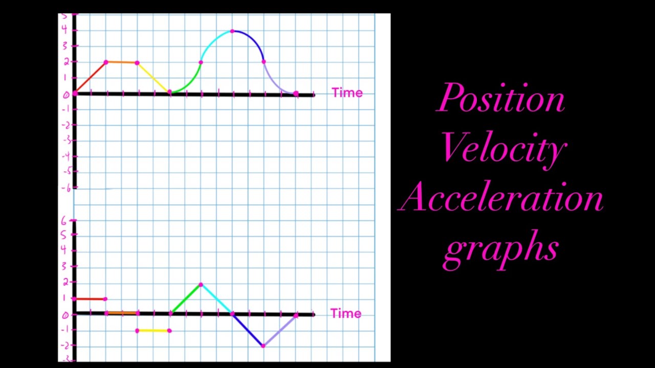
Velocity time graph conversion to Position time graph
TLDRThe lesson focuses on converting velocity-time graphs to position-time graphs. It begins with a review of velocity and position graphs, then explains how to interpret a velocity graph with constant velocity and acceleration. The key is identifying the areas between the x-axis and the graph lines, which represent displacement. The process is demonstrated through three sections of a given velocity graph, with calculations showing how to determine the car's position at different time intervals. The lesson concludes with a practical exercise for the viewer to convert a given velocity graph into a position graph, emphasizing the importance of practice in understanding physics concepts.
Takeaways
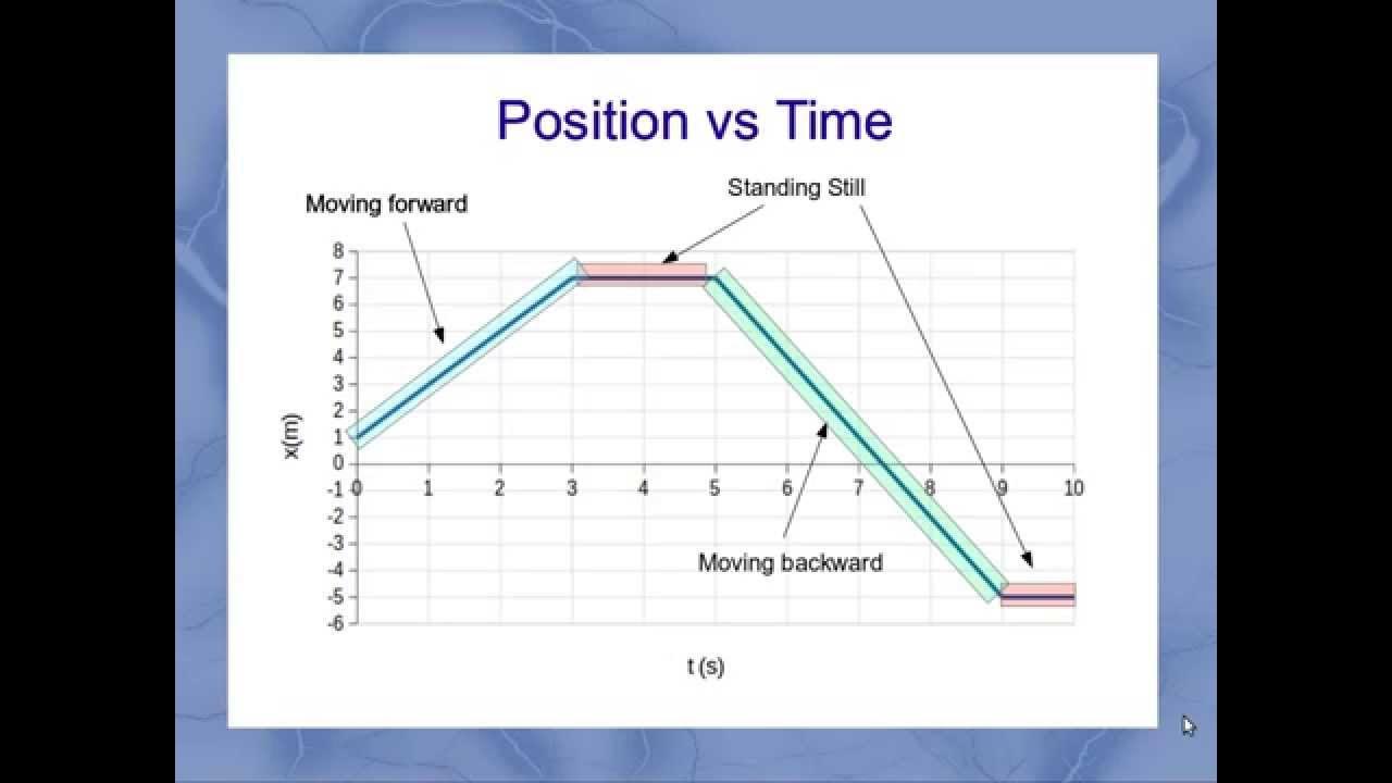
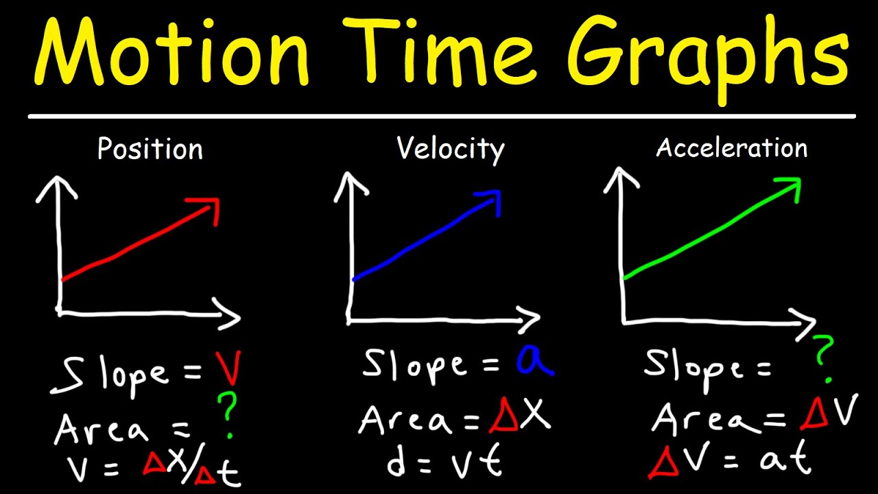
- 📈 The slope of a line on a position-time graph represents velocity.
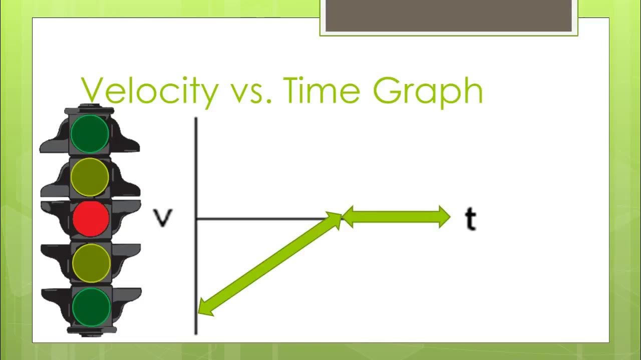
- 📊 A straight line on a velocity-time graph with zero slope indicates no acceleration.
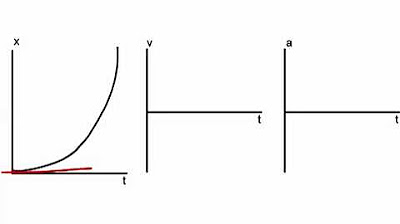
- 🚗 An object's acceleration is represented by the curvature on a position-time graph and the slope on a velocity-time graph.
- 🛣️ In section A (0-4 seconds), the car moves at a constant velocity of 4 m/s north.
- 📉 Section B (4-7 seconds) shows the car slowing down with constant acceleration, moving north.
- 🏁 At the end of section B, the car comes to a stop, indicated by the velocity becoming zero.
- 🔄 The area under the line in a velocity-time graph equals displacement, which is represented as a line on a position-time graph for constant velocity.
- 🔽 Section C (7-10 seconds) depicts the car stopped, represented by the graph line lying on the x-axis.
- 🔄 For constant acceleration, the displacement is calculated as half the product of the average velocity and time interval.
- 🔄 The transition between constant velocity and acceleration must be smooth, maintaining continuity in the slope.
- 📚 Converting a velocity-time graph to a position-time graph involves calculating and representing areas as displacements.
Q & A
What is the initial velocity given to the car in the example?
-The initial velocity given to the car is 4 meters per second.
What does the slope of a line represent on a position-time graph?
-On a position-time graph, the slope of a line represents the velocity of the object.
How is acceleration represented on a position-time graph versus a velocity-time graph?
-On a position-time graph, acceleration is represented by a curve, while on a velocity-time graph, constant acceleration is represented by a straight line.
What is the slope of the line in the velocity-time graph when an object is not accelerating?
-When an object is not accelerating, the slope of the line in the velocity-time graph is exactly zero.
How can you determine if the car is slowing down in section B of the graph?
-In section B, you can determine the car is slowing down by observing that the velocity values are decreasing over time (from 4 m/s to 0 m/s), and the arrow on the graph indicates a decrease in speed.
What is the displacement in section A of the velocity-time graph?
-The displacement in section A is calculated as the area of a rectangle, which is the length (4 seconds) times the width (4 meters per second), resulting in 16 meters.
How is the displacement for section B calculated?
-The displacement for section B is calculated as the area of a triangle, using the formula (1/2) * base * height. The base is 3 seconds and the height is 4 meters per second, resulting in 6 meters of displacement.
Why does the car's velocity remain positive throughout the example, even when it's slowing down?
-The car's velocity remains positive because it is always moving north, and a negative velocity would indicate movement in the opposite direction, which is not the case here.
How do you know the object is stopped in section C of the graph?
-In section C, the object is considered stopped because the velocity is always zero, and the graph line is always on the x-axis, which represents a velocity of 0 meters per second.
What is the significance of a smooth transition in the slope of the graph when moving from constant velocity to slowing down?
-A smooth transition in the slope indicates that the change from constant velocity to slowing down is gradual and not instantaneous, which is physically realistic and expected in most scenarios.
How can you convert a velocity-time graph to a position-time graph?
-To convert a velocity-time graph to a position-time graph, you calculate the area under the velocity curve between the x-axis and the line for each time interval, where the area represents the displacement of the object during that interval.
Outlines
📈 Introduction to Velocity and Position Time Graphs
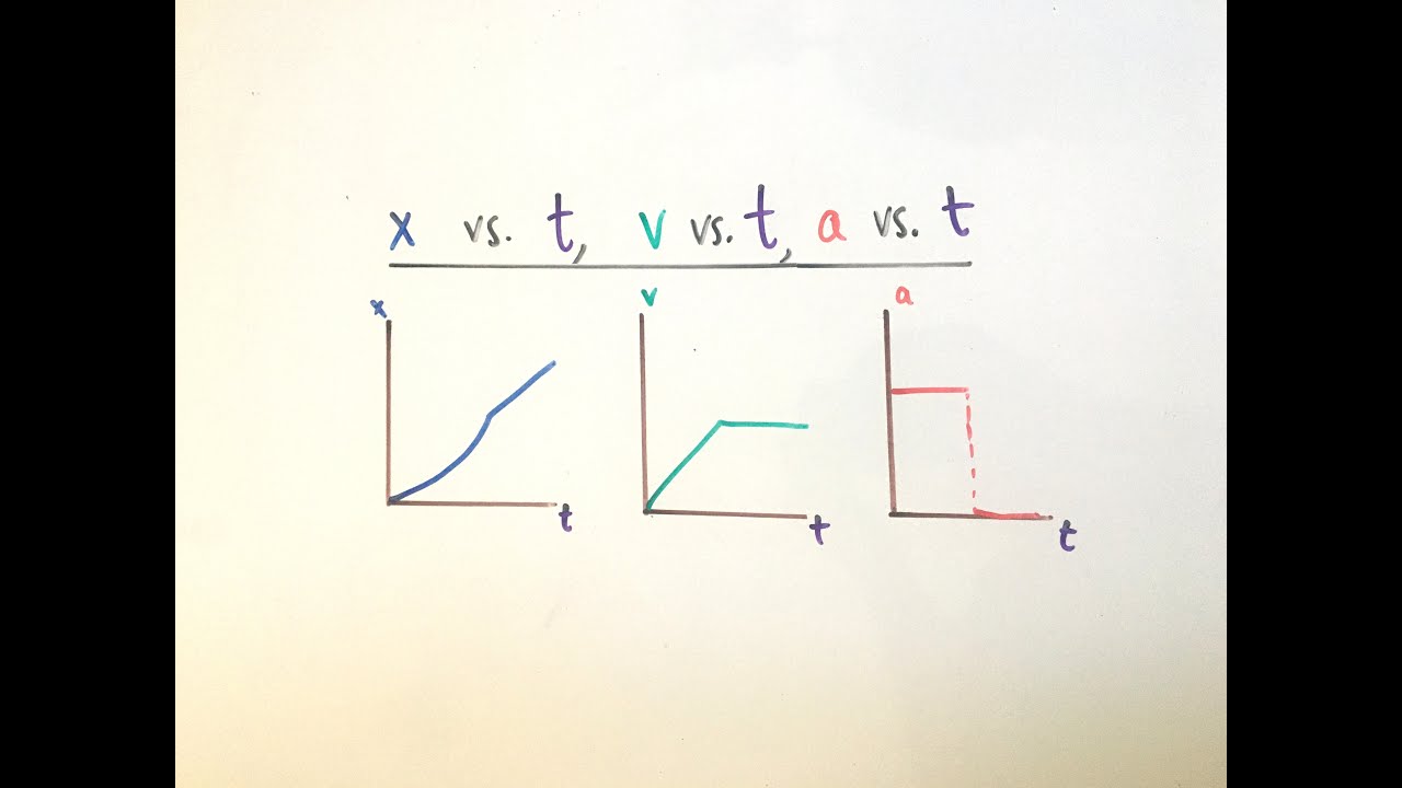
This paragraph introduces the concept of velocity and position time graphs, explaining the basics of how to interpret them. It begins with a review of position and velocity graphs, followed by an example of a car given an initial velocity of 4 meters per second. The explanation details how the position time graph shows a straight line with a slope equal to the velocity, and the velocity time graph shows a line with zero slope when there is no acceleration. The paragraph then discusses the representation of acceleration on both graphs, highlighting the differences between constant acceleration (a straight line) and deceleration (a curve). The car's motion is used as a case study to illustrate these concepts.
📊 Analyzing the Velocity Time Graph in Sections
The paragraph delves into the analysis of a velocity time graph by dividing it into three sections: A, B, and C. Section A (0 to 4 seconds) represents constant velocity, with the car moving north at 4 meters per second. The constant velocity is indicated by the arrow's position at each second. Section B (4 to 7 seconds) shows the car slowing down, moving north, with the velocity decreasing from 4 meters per second to a stop. This is identified by the decreasing numbers on the velocity time graph. Section C (7 to 10 seconds) indicates the car is stopped, as the graph remains on the x-axis. The key takeaway is understanding how to describe the graph's sections and their corresponding motion characteristics.
📐 Creating the Position Time Graph from Velocity Data
This section focuses on the process of converting the velocity time graph into a position time graph. It emphasizes the importance of calculating the area under the curve, which represents displacement. For Section A, the area is calculated as a rectangle, leading to a displacement of 16 meters after 4 seconds. The position time graph then connects the initial position at the origin to the new position using a straight line, reflecting the constant velocity. For Section B, the area is calculated as a triangle, resulting in an additional 6 meters of displacement, and the position time graph uses a curve to represent the car slowing down. The paragraph also introduces the concept of smooth transitions in slope when moving from constant velocity to deceleration. Section C is represented by a straight line on the x-axis, indicating the car is stopped. The exercise encourages the viewer to practice converting the velocity time graph into a position time graph, highlighting the importance of calculating areas and understanding the physical concepts behind the graphs.
🔢 Applying the Formula for Displacement in Section D
The final paragraph introduces Section D, which was not covered in the previous examples, and explains how to draw the area for this section. Section D represents the car traveling south, indicated by a negative velocity at the end of the section. The paragraph uses a formula to calculate the displacement for Section A, where the initial and final velocities are the same, and the time interval is given. The formula is shown to be equivalent to calculating the area under the curve. The paragraph concludes with a summary of the lesson, emphasizing the conversion of a velocity time graph to a position time graph through area calculation and the importance of practice in understanding physics concepts.
Mindmap
Keywords
💡Velocity-Time Graph
💡Position-Time Graph
💡Constant Velocity
💡Acceleration
💡Deceleration
💡Displacement
💡Slope
💡Area Under the Curve
💡Smooth Transition
💡Direction
Highlights
The goal is to interpret a velocity-time graph and convert it into a position-time graph.
A brief review on position and velocity-time graphs is provided.
The car is given an initial velocity of 4 meters per second.
On a position-time graph, the slope represents velocity.
Constant acceleration is represented by a straight line on a velocity-time graph.
The car's motion is divided into three sections (A, B, and C) based on its velocity changes.
Section A (0 to 4 seconds) represents constant velocity with no change in direction.
Section B (4 to 7 seconds) shows the car slowing down with constant acceleration.
Section C (7 to 10 seconds) indicates the car is stopped, with no displacement.
Displacement is calculated by determining the area between the x-axis and the velocity-time graph line.
For constant velocity, the displacement is the product of time and velocity.
For constant acceleration, the displacement is calculated using the formula for the area of a triangle.
The position-time graph starts with the initial position at the origin (zero).
A smooth transition in slope is needed when moving from constant velocity to acceleration.
Section D introduces the concept of the object moving in the opposite direction (south).
The final exercise encourages the audience to convert the velocity-time graph into a position-time graph on their own.
The lesson emphasizes the importance of practice in understanding physics concepts.
The process of converting a velocity-time graph to a position-time graph involves calculating areas for different sections.
Transcripts
Browse More Related Video
Position vs Time, Velocity vs Time & Acceleration vs Time Graph (Great Trick to Solve Every Graph!!)
Kinematics Graphs
Position, Velocity, and Acceleration vs. Time Graphs
Interpreting Motion Graphs
Position/Velocity/Acceleration vs. Time Graphs (AP Physics 1)
Velocity Time Graphs, Acceleration & Position Time Graphs - Physics
5.0 / 5 (0 votes)
Thanks for rating: