Finding the Area Under a Standard Normal Curve Using the TI-84
TLDRThis tutorial demonstrates how to calculate the area under the standard normal curve for given Z-values using a TI-84 calculator. It covers finding the area to the left of Z=0.23, to the right of Z=-1.36, and between Z=-1.23 and Z=1.3. The process involves using the normal CDF function, with bounds set to approximate negative and positive infinity for practical calculation. The tutorial emphasizes the importance of ensuring the calculated areas make sense in the context of the entire area under the curve, which should sum to one.
Takeaways
- 📚 The tutorial explains how to find the area under a standard normal curve using a TI-84 calculator.
- 🔍 The first example demonstrates finding the area to the left of Z = 0.23 on the standard normal curve.
- 📉 The area calculation involves determining the lower and upper bounds of the area under the curve.
- ∞ The lower bound is approximated as negative infinity, using a very small number like -10,000 for practical purposes.
- 🔝 The upper bound for the first example is 0.23, representing the Z value where the area is being calculated.
- 🧮 To calculate the area, use the normal CDF function on the calculator, inputting the bounds in the correct order.
- 📈 The result for the first example is an area of 0.591, which represents 59.1% of the total area under the curve.
- 📊 The second example shows how to find the area to the right of Z = -1.36, using a similar method with the normal CDF function.
- 🔚 For the second example, the result is an area of 0.913, indicating 91.3% of the total area is beyond the Z value.
- 🔄 The third example calculates the area between two Z values, -1.23 and 1.3, using the normal CDF function with these bounds.
- 📐 The area between the two Z values is found to be 0.794, representing approximately 79.4% of the total area.
- 📋 It's important to remember that the total area under the standard normal curve is 1, and the calculated areas should make sense in context.
Q & A
What is the main topic of the tutorial?
-The main topic of the tutorial is how to find the area under a standard normal curve given a Z value using a TI-84 calculator.
What is the first example in the tutorial about?
-The first example is about finding the area under the standard normal curve to the left of Z equals 0.23.
How do you determine the lower and upper bounds for the area under the curve?
-The lower bound is determined by using a very small number, like negative 10,000, to represent negative infinity, and the upper bound is the given Z value.
What function on the TI-84 calculator is used to find the area under the normal curve?
-The normal CDF (Cumulative Distribution Function) is used, which can be accessed by pressing 2nd, then bars, and then selecting number 2.
Why can't negative infinity be used as a lower bound on the calculator?
-Negative infinity cannot be used as a lower bound on the calculator because it is not a numerical value that the calculator can process.
What is the area to the left of Z equals 0.23 in the first example?
-The area to the left of Z equals 0.23 is approximately 0.591.
What is the second example in the tutorial about?
-The second example is about finding the area to the right of Z equals -1.36.
How do you represent positive infinity on the calculator for the second example?
-Positive infinity is represented by using a large number, like 10,000, on the calculator.
What is the area to the right of Z equals -1.36 in the second example?
-The area to the right of Z equals -1.36 is approximately 0.913.
What is the third example in the tutorial about?
-The third example is about finding the area between Z equals -1.23 and Z equals 1.3.
What is the area between Z equals -1.23 and Z equals 1.3 in the third example?
-The area between Z equals -1.23 and Z equals 1.3 is approximately 0.794.
Why is it important to check if the calculated area makes sense?
-It is important to check if the calculated area makes sense because the entire area under the standard normal curve should equal 1, and the calculated areas should be a reasonable proportion of this total area.
Outlines
📊 Calculating Area Under Standard Normal Curve
This paragraph introduces a tutorial on calculating the area under a standard normal curve given a Z-score using a TI-84 calculator. The focus is on finding the area to the left of Z=0.23, which is explained as being from negative infinity up to 0.23. The method involves using the normal cumulative distribution function (CDF) accessible through the calculator's menu. The tutorial suggests using a very small number like -10,000 as a substitute for negative infinity and demonstrates the process of inputting the lower and upper bounds to find the area, which in this case is approximately 0.591.
Mindmap
Keywords
💡Area under the curve
💡Standard normal curve
💡Z value
💡TI-84 calculator
💡Normal CDF function
💡Lower bound
💡Upper bound
💡Negative infinity
💡Positive infinity
💡Probability
💡Graphical representation
Highlights
Tutorial on finding the area under the standard normal curve for a given Z value using the TI-84 calculator.
Explanation of how to determine the lower and upper bounds for calculating the area under the curve.
Using the normal CDF function on the TI-84 to find the area to the left of Z equals 0.23.
Substituting negative infinity with a very small number like -10,000 for practical calculation purposes.
Calculation of the area to the left of Z equals 0.23 resulting in 0.591.
Finding the area to the right of Z equals -1.36 using the normal CDF function.
Using -100,000 as a substitute for negative infinity in the calculator for more precision.
Calculation of the area to the right of Z equals -1.36 resulting in 0.913.
Method for calculating the area between two Z values, -1.23 and 1.3.
Direct input of Z values into the normal CDF function for the area between -1.23 and 1.3.
Result of the area between -1.23 and 1.3 is 0.794, indicating the majority of the data distribution.
Emphasis on the total area under the standard normal curve summing up to one.
Suggestion to visually inspect the graph to ensure the calculated areas make sense.
Highlighting the importance of understanding the practical implications of the calculated areas.
Explanation of how the calculated areas relate to percentages of the total data distribution.
Visual inspection tips to verify the accuracy of the calculated areas.
Final summary of the tutorial's main points and their significance in statistical analysis.
Transcripts
Browse More Related Video
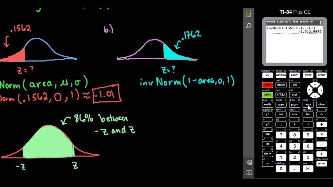
Finding Z-score Given Area - TI-84
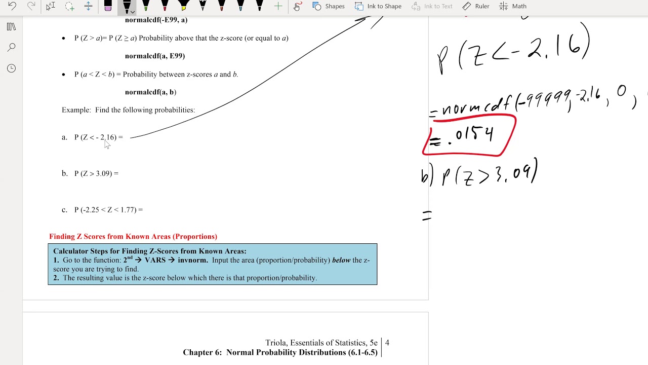
Math 119 Chap 6 part 1
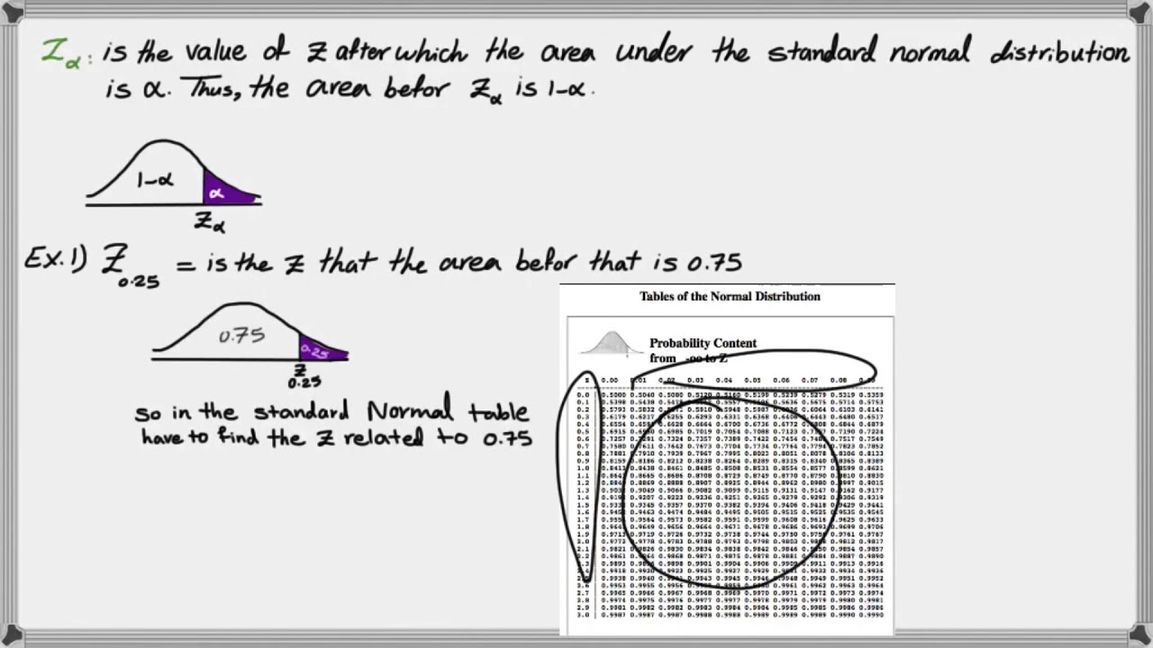
How to find critical Z value (Z alpha)

Find the z-score given the confidence level

Z-Scores, Standardization, and the Standard Normal Distribution (5.3)
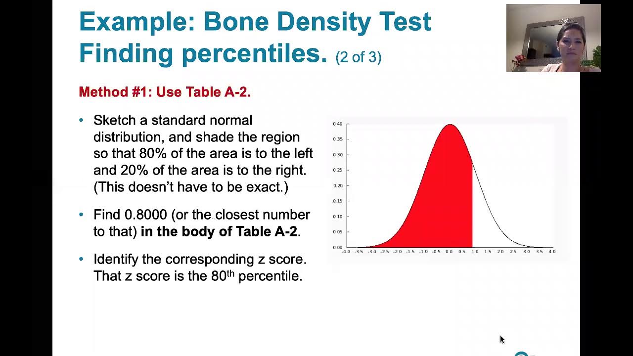
6.1.5 Standard Normal Distribution - z scores Corresponding to Areas. Percentiles. Critical Values.
5.0 / 5 (0 votes)
Thanks for rating: