Math 119 Chap 6 part 1
TLDRThis instructional video introduces Chapter Six, focusing on normal distribution in statistics. The instructor explains the concept of a normal distribution, its attributes like symmetry and bell shape, and the significance of the total area under the curve equating to one. Emphasizing the use of calculators for complex calculations, the video demonstrates how to find probabilities using z-scores and the normal cumulative distribution function (normalcdf) on a TI-84 Plus calculator. The session includes practical examples to help students understand the calculation of probabilities for z-scores being less than, greater than, or between specific values.
Takeaways
- 🎥 The video is an introduction to Chapter 6 of a course, focusing on normal distribution and z-scores.
- 🕒 The video is expected to be around 20 to 30 minutes long to help students get accustomed to the format.
- 📈 The instructor emphasizes the importance of the normal distribution's symmetric, bell-shaped graph and its formula involving 'e to the power of...'.
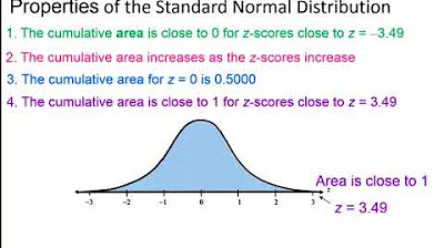
- 📊 The total area under the normal distribution curve equals one, representing 100%, which is crucial for understanding probabilities.
- 📚 Students are advised to have chapters 1 through 6 printed out for reference during the video.
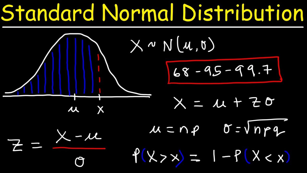
- 📉 The empirical rule is mentioned as a method for approximating probabilities in a normal distribution, with the 68-95-99.7 percentages.
- 🔢 The standard normal distribution is defined with a mean (mu) of zero and a standard deviation (sigma) of one.
- ⚖️ Z-scores are explained as a measure of relative standing in comparison to the mean, indicating how many standard deviations away from the mean a value is.
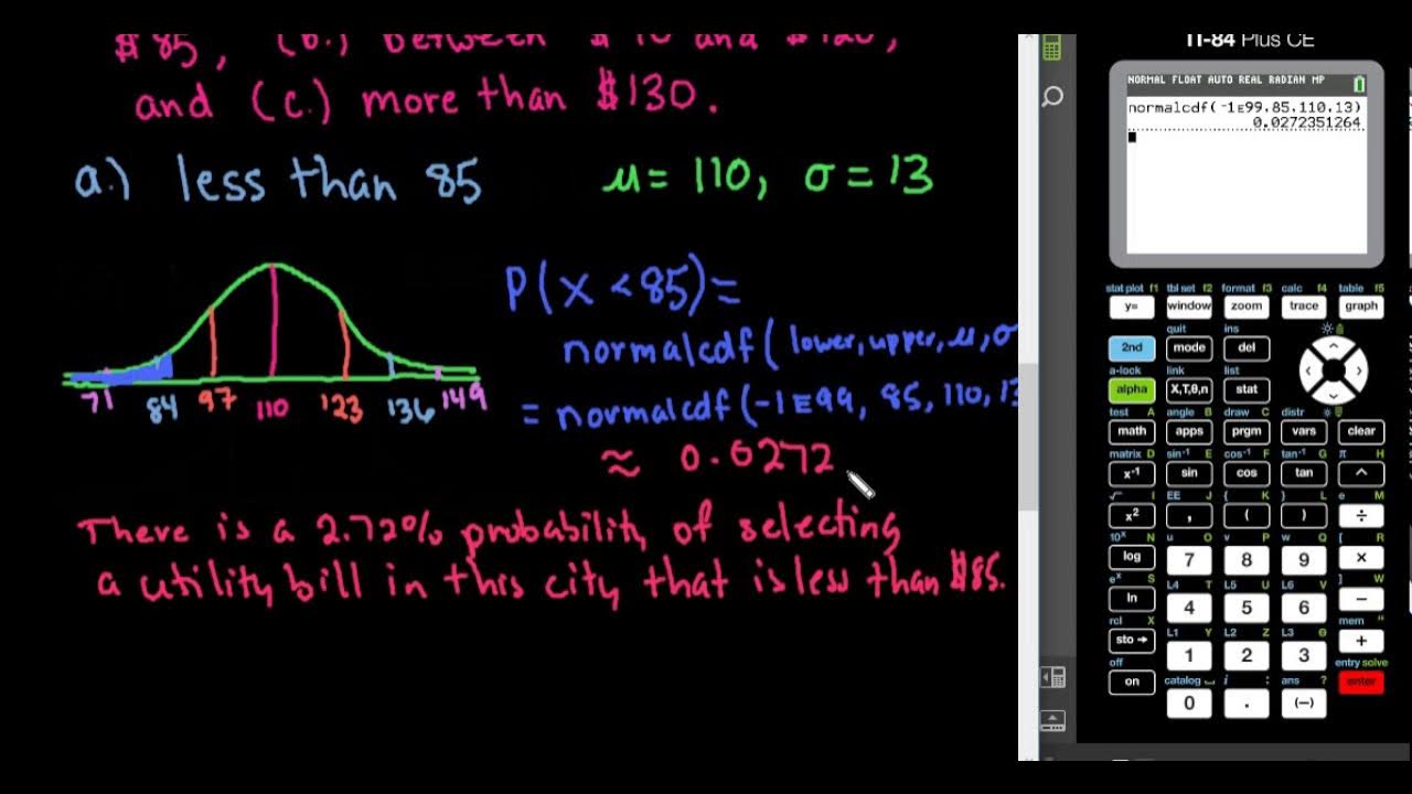
- 🧮 The use of a calculator, specifically the 'normalcdf' function on a TI-84 Plus, is highlighted for finding probabilities associated with z-scores.
- 📝 The instructor provides step-by-step instructions on how to use the calculator for different probability scenarios involving z-scores.
- 🔍 The video script includes practical examples of calculating probabilities for z-scores being less than, greater than, and between certain values.
Q & A
What is the main focus of the first video from chapter six?
-The main focus of the first video is to introduce the concept of normal distribution, its attributes, and the use of calculators for calculations related to it.
What are the key attributes of a normal distribution mentioned in the script?
-The key attributes of a normal distribution are that it is symmetric, has a single peak (one mode), is bell-shaped, and the total area under the curve equals one (100%).
Why is the formula for a normal distribution not a primary concern in this context?
-The formula for a normal distribution is not a primary concern because the calculations will be done using a calculator, emphasizing the understanding of the distribution's characteristics and the use of technology for computation.
What is the empirical rule and how does it relate to the normal distribution?
-The empirical rule is a way to approximate probabilities of a normal distribution using the percentages 68%, 95%, and 99.7%, which represent the area under the curve within one, two, and three standard deviations from the mean, respectively.
What is a z-score and how does it relate to the standard normal distribution?
-A z-score indicates the relative standing of a data point compared to the mean, measured in terms of standard deviations. In the context of the standard normal distribution, a z-score always has a mean of zero and a standard deviation of one.
What is the purpose of the normalcdf function on the calculator?
-The normalcdf function on the calculator is used to find the cumulative distribution function (CDF) for a normal distribution, which helps in determining the probability of a z-score being less than, greater than, or between certain values.
How does the instructor plan to handle office hours for the course?
-The instructor plans to have set times for office hours, where students can discuss parts of the course they didn't understand, presumably through the Zoom platform.
What is the significance of the area under the normal density curve in terms of probabilities?
-The area under the normal density curve represents the probability of a particular event occurring. Since the total area is one (or 100%), it allows for the discussion of probabilities in terms of the area under the curve.
What is the standard normal distribution and why is it important?
-The standard normal distribution is a normal distribution with a mean (mu) of zero and a standard deviation (sigma) of one. It is important because it serves as a basis for comparing other normal distributions and for calculating probabilities using z-scores.
How does the instructor plan to approach the teaching of z-scores in the course?
-The instructor plans to focus heavily on z-scores, teaching how to interpret them in the context of a normal distribution as probabilities, and how to calculate them using the formula x minus mu over the standard deviation.
What is the formula for calculating a z-score mentioned in the script?
-The formula for calculating a z-score is (x - mu) / sigma, where x is the data point, mu is the mean, and sigma is the standard deviation.
Outlines
📚 Introduction to Chapter Six and Normal Distribution
The instructor begins the first video of Chapter Six, introducing the format of 20-30 minute videos and the plan for office hours to discuss any difficulties. The main focus is on the normal distribution, characterized by its symmetric, bell-shaped graph and the formula involving 'e to the power of...'. The instructor emphasizes the importance of the area under the curve representing probabilities and the attributes of a normal distribution, such as being symmetric, having a single peak, and the total area equating to one. The standard normal distribution is also introduced with its specific parameters (mean=0, standard deviation=1) and the concept of z-scores for measuring relative standing to the mean.
🔢 Calculator Steps for Finding Probabilities of Z-Scores
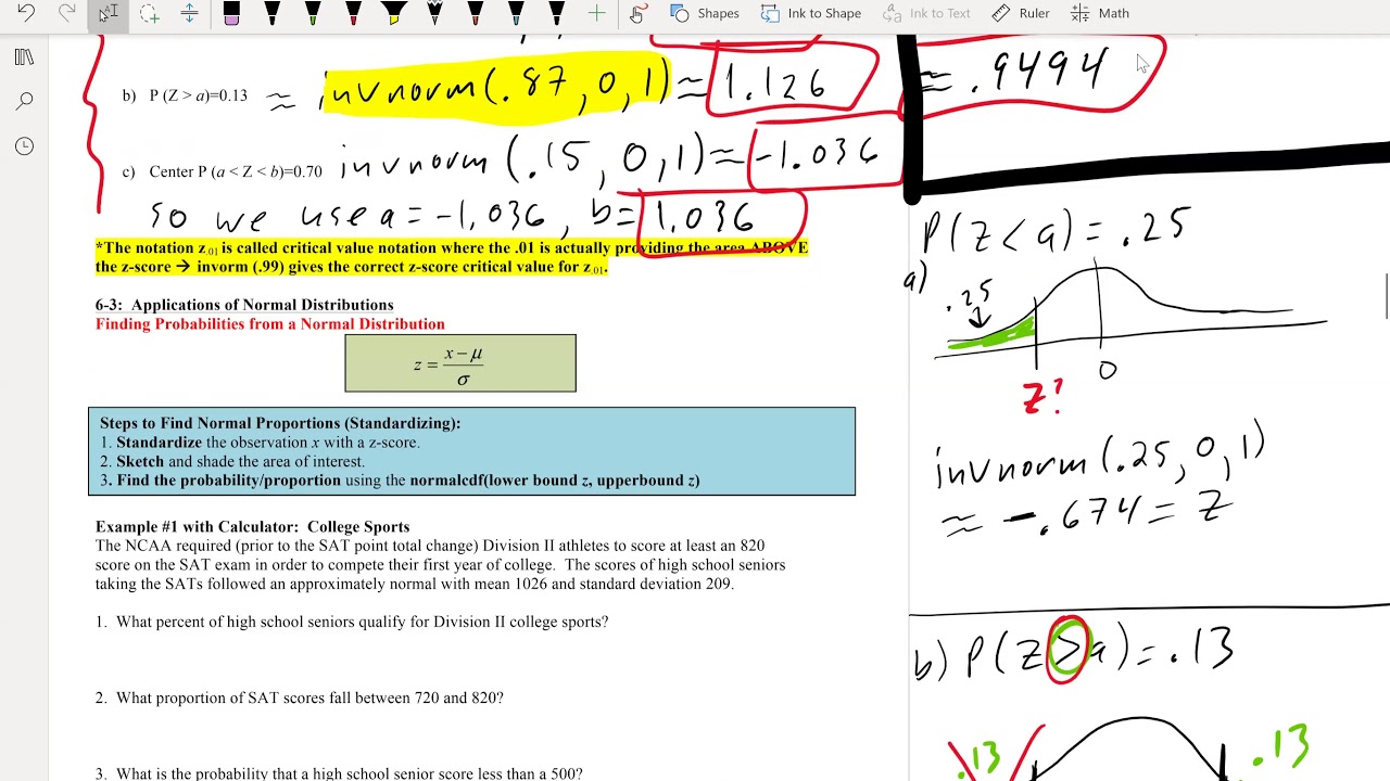
The instructor explains the process of using a calculator, specifically the TI-84 Plus, to find probabilities associated with z-scores. The focus is on using the 'normalcdf' function, which calculates the cumulative distribution function for the normal distribution. The video demonstrates how to find the probability of a z-score being less than a certain value by setting the lower bound to a very negative number and the upper bound to the z-score of interest. The example provided calculates the probability of a z-score being less than -2.16, resulting in approximately 0.0154.
📉 Understanding Z-Score Probabilities and Empirical Rule
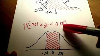
The video continues with the calculation of probabilities for z-scores greater than a certain value and the probability of a z-score falling between two values. The instructor uses the empirical rule, which approximates probabilities based on the standard normal distribution, and the concept of z-scores to explain the calculations. The example for part b calculates the probability of a z-score being greater than 3.09, which is found to be very small, approximately 0.001. The instructor also discusses the importance of visualizing the z-scores on the normal distribution curve to understand the areas and probabilities better.
📝 Conclusion and Homework Preview
The instructor wraps up the video by summarizing the key points covered, including using calculators to find areas to the right, left, or in between two z-scores on the normal distribution curve. The video serves as an introduction to the homework, which will be posted soon, and encourages students to practice the examples provided. The instructor also reassures students that they will become more comfortable with the process as they continue with the course and looks forward to further discussions on Monday.
Mindmap
Keywords
💡Normal Distribution
💡Calculator
💡Empirical Rule
💡Z-Score
💡Standard Normal Distribution
💡Cumulative Distribution Function (CDF)
💡Continuous Random Variable
💡Symmetric
💡Mean
💡Standard Deviation
💡Area Under the Curve
Highlights
Introduction to the first video from chapter six with an expected duration of 20-30 minutes.
Announcement of future course structure with Zoom videos and set office hours for discussion.
Emphasis on the importance of the normal distribution formula and its characteristics such as symmetry and bell shape.
Explanation of the attributes of a normal distribution including single peak, bell-shaped curve, and total area under the curve equals one.
Clarification that the area under the normal density curve represents probabilities.
Brief mention of the uniform distribution and its equal probability across all values.
Discussion on the importance of the density curve in describing the pattern of a continuous distribution.
Introduction of the empirical rule and its use in approximating probabilities of a normal distribution.
Definition of the standard normal distribution with mean (mu) equal to zero and standard deviation (sigma) equal to one.
Explanation of the z-score as a measure of relative standing in comparison to the mean.
Focus on the use of calculators for normal distribution calculations rather than manual computation.
Instruction on using the normalcdf function on calculators for finding probabilities associated with z-scores.
Demonstration of how to calculate the probability of a z-score being less than a specific value using the calculator.
Illustration of calculating the probability of a z-score being greater than a specific value.
Method for finding the probability of a z-score falling between two given values.
Encouragement for students to practice using calculators to solve problems from the upcoming homework.
Closing remarks with an invitation for students to get comfortable with the Zoom platform and look forward to further discussions on Monday.
Transcripts
Browse More Related Video
Math 119 Chap 6 part 2
Elementary Statistics - Chapter 6 Normal Probability Distributions Part 1
Probabilities in a Normal Distribution - TI-84

Elementary Stats Lesson #11
Stats: Finding Probability Using a Normal Distribution Table
Standard Normal Distribution Tables, Z Scores, Probability & Empirical Rule - Stats
5.0 / 5 (0 votes)
Thanks for rating: