7.1.3 Estimating a Population Proportion - Critical Values, Rationale and How to Compute Them
TLDRThis educational video script delves into the concept of critical values and their role in estimating population proportions with confidence intervals. It explains the normal distribution of sample proportions, how to compute their mean and standard deviation, and the significance of the z-score in determining critical values for different confidence levels. The script guides viewers through calculating the critical value for an 86% confidence level using both standard normal distribution methods and practical tools like Excel, emphasizing the importance of these statistical measures in data analysis.
Takeaways
- 📚 The video discusses learning outcome number three from lesson 7.1, focusing on the rationale behind the definition of a critical value and computing critical values for a given confidence level.
- 🔍 It emphasizes estimating a population proportion 'p' by creating a sampling distribution of sample proportions, which involves selecting random samples from the original population and calculating the proportion 'p-hat' for each sample.
- 📉 The script explains that the distribution of sample proportions tends to have a normal distribution, which is a key concept in statistical inference.
- 🎯 The mean of the sampling distribution of sample proportions is equal to the population proportion 'p', making 'p-hat' an unbiased estimator of 'p'.
- 📏 The standard deviation of 'p-hat' can be approximated using the formula √(p-hat * q-hat / n), where 'q-hat' is one minus 'p-hat', and 'n' is the sample size.
- 🌐 The script introduces the concept of converting a non-standard normal distribution to a standard normal distribution to facilitate the computation of critical values.
- 🔑 Critical values are defined as the z-scores that separate the most likely values of 'p-hat' (those within the confidence interval) from the significantly high or low values.
- 📊 For a given confidence level, the critical value 'z-sub-alpha-over-2' is the z-score that has an area of 'alpha/2' to the right, with 'alpha' being the significance level (1 - confidence level).
- 📈 The video provides a step-by-step method to find the critical value for a specific confidence level, using both technology (e.g., Excel) and statistical tables.
- 📝 Common confidence levels like 90%, 95%, and 99% have standard critical values (1.645, 1.96, and approximately 2.576, respectively), which are often memorized or quickly looked up in statistical tables.
- 🔍 The video concludes with a practical example of finding the critical value for an 86% confidence level, demonstrating the process of using Excel's NORM.S.INV function and statistical tables to determine the z-score.
Q & A
What is the main topic discussed in the video script?
-The main topic discussed in the video script is the concept of critical values in the context of estimating a population proportion, including the rationale behind their definition and how to compute them for a given confidence level.
What is a sampling distribution of sample proportions?
-A sampling distribution of sample proportions is a distribution that shows all possible sample proportions (p-hats) obtained by repeatedly selecting samples of the same size from the original population and calculating the proportion for each sample.
Why is the sampling distribution of sample proportions important in estimating the population proportion?
-The sampling distribution of sample proportions is important because it allows us to infer characteristics about the population proportion. It is an unbiased estimator, meaning its mean is equal to the population proportion, which is what we aim to estimate.
What is the relationship between the mean of the sampling distribution of sample proportions and the population proportion?
-The mean of the sampling distribution of sample proportions is equal to the population proportion. This relationship is crucial because it indicates that the sample proportions are good, unbiased estimators of the population proportion.
How is the standard deviation of the sample proportions estimated?
-The standard deviation of the sample proportions is estimated using the formula \( \sqrt{\frac{\hat{p}(1-\hat{p})}{n}} \), where \( \hat{p} \) is the sample proportion and \( n \) is the sample size.
What is the significance of the critical value in the context of confidence intervals?
-The critical value is significant because it separates the range of values of the sample proportion that are considered not significantly high or low from those that are. It helps define the confidence interval by indicating the boundaries within which the population proportion is likely to fall.
How is the critical value denoted mathematically in the context of a confidence interval?
-The critical value is denoted as \( z_{\alpha/2} \), which represents the z-score that corresponds to the tail area of \( \alpha/2 \) in a standard normal distribution.
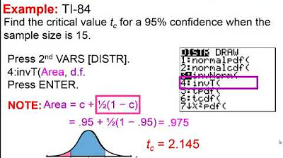
What is the process of finding the critical value corresponding to an 86% confidence level?
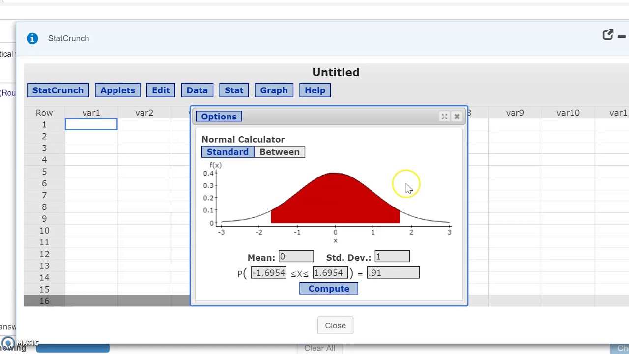
-To find the critical value for an 86% confidence level, you would sketch a standard normal distribution with 86% of the area in the middle, compute \( \alpha \) as 14% and divide it by 2 to get 7% for each tail. Then, find the z-score that has an area of 0.93 to the left, which can be done using technology like Excel or a standard normal distribution table.
How can the critical value be found using Excel?
-In Excel, you can find the critical value by using the NORM.S.INV function, which gives the inverse of the standard normal distribution. You input the area to the left (probability), which in this case would be 0.93, and Excel returns the corresponding z-score.
What are the most common confidence levels and their corresponding critical values?
-The most common confidence levels are 90%, 95%, and 99%, with corresponding critical values of approximately 1.645, 1.96, and 2.576, respectively. These values are often memorized or quickly looked up in standard normal distribution tables.
Why might a non-standard normal distribution be converted to a standard normal distribution?
-A non-standard normal distribution might be converted to a standard normal distribution to simplify calculations, especially when dealing with z-scores and finding critical values for confidence intervals.
Outlines
📚 Introduction to Critical Values and Sample Proportions
This paragraph introduces the concept of critical values in the context of estimating a population proportion, p. It explains the process of creating a sampling distribution of sample proportions by randomly selecting values from the original population, computing the proportion for each sample, and repeating this process to form a distribution. The mean of this distribution is identified as the population proportion p, making it an unbiased estimator. The standard deviation of the sample proportions is discussed as an approximation, which is crucial for understanding the distribution's spread. The paragraph sets the stage for further exploration of critical values and their role in statistical inference.
📉 Understanding Confidence Intervals and Critical Values
The second paragraph delves into the concept of confidence intervals, focusing on the significance of sample proportions (p-hat) and how they relate to the population proportion (p). It discusses the conversion of a non-standard normal distribution to a standard normal distribution and the process of identifying significant values of p-hat by separating them from non-significant ones using a confidence interval. The critical value, denoted as z-sub-alpha-over-2, is defined as the z-score that separates the significant values from the non-significant ones in the distribution. The paragraph provides an example of finding the critical value for an 86% confidence level, illustrating the steps involved in calculating and interpreting this value.
🔍 Calculating the Critical Value for a Given Confidence Level
This paragraph provides a step-by-step guide on calculating the critical value for a specified confidence level, using both Excel and a standard normal distribution table. It explains the process of sketching a standard normal distribution, determining the area under the curve for the confidence level, and finding the corresponding z-score that separates the significant tail area from the central area. The example given is for an 86% confidence level, showing how to calculate the z-score using the area to the left of z-sub-alpha-over-2. The paragraph also demonstrates how to use Excel's NORMSINV function and a standard normal distribution table to find the critical value, reinforcing the understanding of critical values in statistical analysis.
📈 Common Confidence Levels and Their Associated Critical Values
The final paragraph discusses the most commonly used confidence levels, such as 90%, 95%, and 99%, and their corresponding critical values. It explains how to find these critical values using a standard normal distribution table, with a focus on the z-scores for the 95% and 99% confidence levels, which are 1.96 and approximately 2.576, respectively. The paragraph also highlights the convenience of using a table for quick reference to these common critical values, streamlining the process of statistical analysis for researchers and statisticians.
Mindmap
Keywords
💡Critical Value
💡Confidence Level
💡Sample Proportion (p-hat)
💡Sampling Distribution
💡Population Proportion (p)
💡Standard Deviation
💡Normal Distribution
💡Z-Score
💡Alpha (α)
💡Margin of Error
Highlights
The video discusses learning outcome number three from lesson 7.1, focusing on the rationale behind defining a critical value and computing critical values for a given confidence level.
The lesson is about estimating a population proportion, p, using the distribution of sample proportions from the original population.
Sampling distributions of sample proportions are created by repeatedly selecting random samples and computing the proportion for each.
Sample proportions tend to have a normal distribution, which is crucial for statistical inference.
The mean of the sampling distribution of sample proportions is equal to the population proportion, making it an unbiased estimator.
The standard deviation of the sample proportions can be estimated using the formula √(p̂(1-p̂)/n).
Continuous random variables' distributions are represented by probability density functions, with areas under the curve representing probabilities.
Confidence intervals separate the most likely values of the sample proportion from those considered significantly high or low.
Critical values are z-scores that separate the middle area of the distribution from the tails, representing non-significant values.
The critical value zα/2 is used to find the z-score with an area of α/2 to the right, corresponding to a specific confidence level.
An example is given to find the critical value for an 86% confidence level, involving calculating α and using it to find the corresponding z-score.
Excel's NORM.S.INV function is demonstrated to find the z-score for a given area to the left.
Table A2 is used to find the critical values for common confidence levels, such as 90%, 95%, and 99%.
The video provides a step-by-step guide on how to calculate and interpret critical values for different confidence levels.
The importance of understanding the distribution of sample proportions and their relation to the population proportion is emphasized.
The video concludes with a preview of the next topic, the margin of error, which is integral to constructing confidence intervals.
Transcripts
Browse More Related Video
Elementary Statistics - Chapter 7 - Estimating Parameters and Determining Sample Sizes Part 2
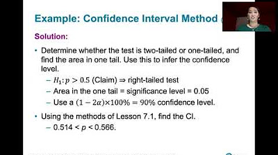
8.2.2 Testing a Claim About A Proportion - Confidence Interval Method, Comparison to Other Methods

Elementary Stats Lesson #16
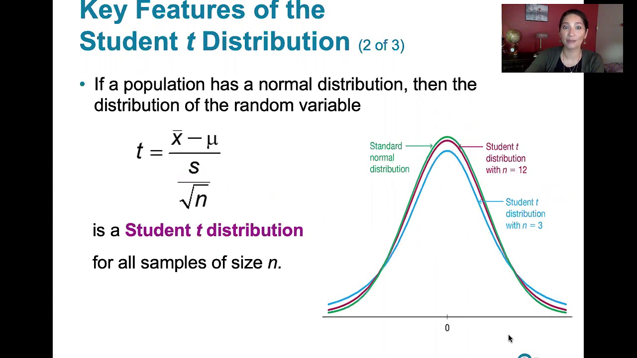
7.2.1 Estimating a Population Mean - Student t Distribution and Finding Critical t Values
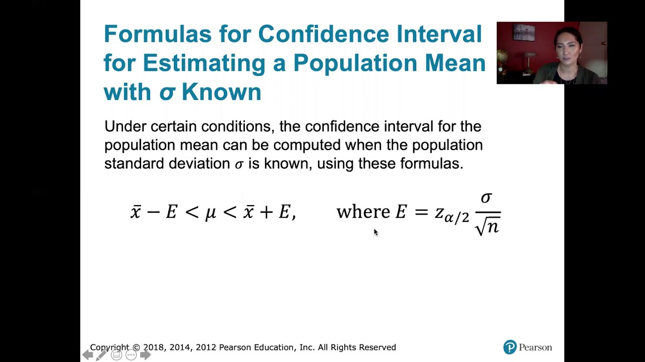
7.2.5 Estimating a Population Mean - Confidence Intervals with Known Pop. Standard Deviation
Find Critical Value Za/2 with Statcrunch
5.0 / 5 (0 votes)
Thanks for rating: