Elementary Statistics - Chapter 7 - Estimating Parameters and Determining Sample Sizes Part 2

Joan DeRosa

15 Oct 201723:49

EducationalLearning

32 Likes 10 Comments

TLDRThis video script provides a comprehensive tutorial on constructing confidence intervals, focusing on the use of t-distribution when the population standard deviation is unknown and the sample size is less than 30. It explains the conditions for choosing between t-distribution and z-distribution, calculating degrees of freedom, and finding critical values using tables or calculators. The script also covers estimating population proportions, constructing confidence intervals for proportions, and determining minimum sample sizes for given confidence levels and margins of error, using examples to illustrate the concepts.

Takeaways

📊 When estimating the mean and the population standard deviation is unknown, and the sample size is less than 30, use the t-distribution to find the critical value T.
🔢 The critical values of T are denoted by T_sub_C and are found using calculators or distribution tables based on the confidence level.
🎯 To choose between the T or Z distribution, consider if the population standard deviation is known and if the sample size is greater than 30.
🔄 The degree of freedom (DF) is calculated as the sample size minus one and is used to account for discrepancies in standard deviation values.
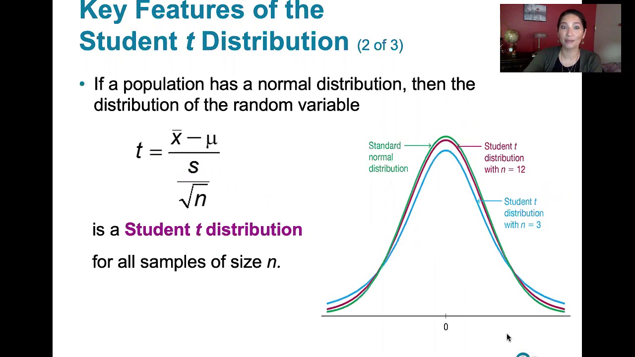
📚 As sample size increases, the T distribution approaches the Z distribution, especially when the sample size is greater than 100.
🔍 To find the critical value for T at a 95% confidence level with a sample size of 15, use the degree of freedom (14 in this case) and refer to the t-distribution table or calculator.
📝 Never get a negative T distribution value; ensure to incorporate the tail area when calculating critical values using a calculator.
🌡️ An example provided involves constructing a 95% confidence interval for the mean temperature of coffee in 16 shops, using the t-distribution with a sample mean and standard deviation.
📲 For population proportions, estimate P (probability of success) using P_hat, calculated as the number of successes over the sample size.
📉 To construct a confidence interval for a population proportion, ensure the product of the sample size and P_hat or Q_hat (1 - P_hat) is at least 5.
🔢 The minimum sample size needed for estimating the population proportion with a given confidence level and margin of error can be calculated using a specific formula, rounding up to the nearest whole number.

Q & A

What is the main difference between using the T-distribution and the Z-distribution for confidence intervals?
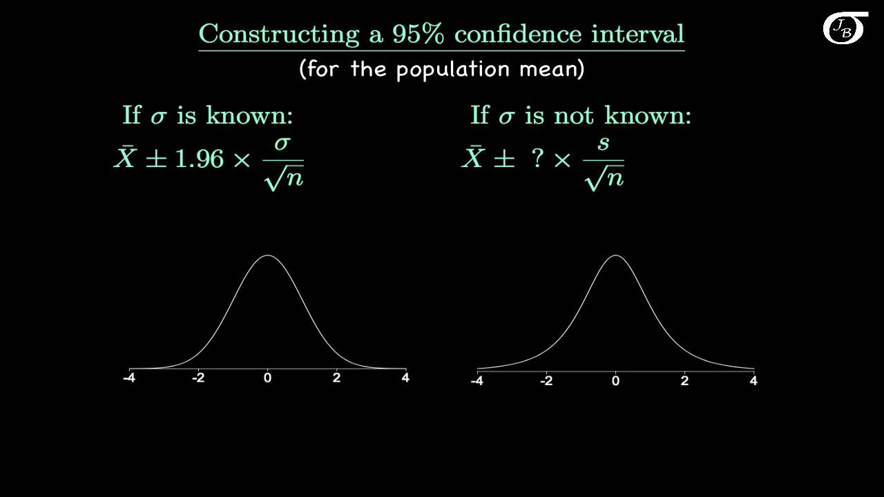
-The main difference is that the T-distribution is used when the population standard deviation is unknown and the sample size is less than 30, while the Z-distribution is used when the population standard deviation is known or when the sample size is greater than 30.
What is the formula to calculate the critical value for the T-distribution?
-The critical value for the T-distribution is found using the T-table or a calculator, denoted by T_sub_C, and is based on the degree of freedom (DF) and the confidence level.
How is the degree of freedom (DF) calculated in the context of the T-distribution?
-The degree of freedom is calculated as the sample size minus one (DF = n - 1), and it accounts for the estimation of the population standard deviation from the sample.
Under what conditions would you choose to use the Z-distribution over the T-distribution?
-You would choose the Z-distribution if the population standard deviation is known and the sample size is greater than 30, indicating a normally distributed population.
What is the significance of the critical value T_sub_C in constructing confidence intervals?
-The critical value T_sub_C is used to determine the boundaries of the confidence interval and is dependent on the chosen confidence level and the degree of freedom.
How do you find the 95% confidence interval for the mean temperature of coffee in a sample of 16 coffee shops?
-You would calculate the sample mean, use the sample standard deviation, and apply the T-distribution with a degree of freedom of 15 to find the critical value and construct the interval.
What is the formula for calculating the margin of error in a confidence interval for a proportion?
-The margin of error is calculated using the formula: Margin of Error = Z_critical * sqrt((p_hat * (1 - p_hat)) / n), where p_hat is the sample proportion, n is the sample size, and Z_critical is the Z-score corresponding to the confidence level.
How do you determine the minimum sample size needed for a given confidence level and margin of error?
-The minimum sample size is determined using the formula: n = (Z_critical * sqrt((p_hat * (1 - p_hat)) / E))^2, where E is the margin of error expressed as a decimal, and Z_critical is the Z-score for the desired confidence level.
What is the point estimate for a population proportion, and how is it calculated?
-The point estimate for a population proportion, denoted as p_hat, is calculated as the number of successes (x) divided by the sample size (n), and it represents the best guess of the true population proportion based on the sample data.
Why is it important to round up the calculated sample size when determining the minimum sample size needed for a study?
-Rounding up ensures that the sample size is large enough to provide the desired level of confidence and precision in the study, as you cannot have a fraction of a participant in a sample.

Outlines

00:00

📊 Understanding T-Distribution and Confidence Intervals

This paragraph introduces the concept of confidence intervals for the mean when the population standard deviation is unknown and the sample size is less than 30. It explains the use of the t-distribution in such cases, as opposed to the Z-distribution, which is used when the population standard deviation is known and the sample size is greater than 30. The paragraph details the process of finding critical values for the t-distribution using either a calculator or a distribution table, and emphasizes the importance of understanding when to use the t-distribution versus the Z-distribution. It also discusses the concept of degrees of freedom and how they relate to the sample size, noting that as the sample size increases, the t-distribution approaches the Z-distribution.

05:02

📚 Calculating the T-distribution Critical Value and Confidence Intervals

The second paragraph delves into the specifics of calculating the critical value for the t-distribution using both a t-distribution table and a calculator. It explains the process of finding the area under the curve that represents the confidence level and incorporating the tail area that is not shaded. The paragraph provides an example of constructing a confidence interval for the mean temperature of coffee from a sample of 16 coffee shops, using the sample mean, standard deviation, and the t-distribution to find the interval. It also discusses the importance of entering the correct values into the calculator and the steps involved in using the calculator to find the confidence interval.

10:02

📉 Estimating Population Proportions and Confidence Intervals

This paragraph shifts focus to estimating population proportions using sample proportions. It explains the point estimate for a proportion, denoted as P hat, which is calculated as the number of successes divided by the sample size. The paragraph also covers the calculation of Q hat, the estimate for the failure percentage. It discusses the rounding rules for interval estimates of proportions and provides an example of a survey where 662 out of 1000 US adults find it acceptable to check personal emails at work, illustrating how to calculate P hat and Q hat. The paragraph also outlines the steps for manually constructing a confidence interval for a population proportion, emphasizing the importance of ensuring the sample size times P hat and Q hat are both greater than or equal to five.

15:03

🔢 Determining Minimum Sample Size for Estimating Population Proportions

The fourth paragraph discusses the formula for determining the minimum sample size needed to estimate a population proportion with a given confidence level and margin of error. It explains the importance of using a preliminary estimate for P hat if available, and if not, using 0.5 for both P hat and Q hat. The paragraph provides a step-by-step guide on how to use the formula, including finding the critical value Z based on the confidence level and incorporating it into the formula. It also emphasizes the need to always round up to the nearest whole number when calculating the minimum sample size, providing examples of calculating the minimum sample size for a political campaign with and without a preliminary estimate.

20:05

📝 Examples of Calculating Minimum Sample Size for Political Campaigns

The final paragraph provides two examples of calculating the minimum sample size for a political campaign, one without a preliminary estimate and one with a given P hat of 0.31. It explains the process of finding the critical Z value for a 95% confidence level and a 3% margin of error, and then using this value in the formula to calculate the minimum sample size. The paragraph illustrates the importance of using the correct values and rounding up to ensure an accurate and sufficient sample size. It concludes with the calculated minimum sample sizes of 1068 and 914 voters for the two scenarios, respectively.

Mindmap

Keywords

💡Confidence Interval

A confidence interval is a range within which we expect the true population parameter to lie, with a certain level of confidence. In the video, confidence intervals are used to estimate the mean temperature of coffee, the population mean commute time, and the repair costs, providing a range of values that are likely to contain the true mean with a 95% level of confidence.

💡T-Distribution

The T-distribution, also known as Student's T-distribution, is a type of probability distribution that is used when the sample size is small and the population standard deviation is unknown. The video script explains that when the sample size is less than 30 and the variable is approximately normally distributed, the T-distribution is used to find critical values for constructing confidence intervals.

💡Population Standard Deviation

The population standard deviation is a measure of the amount of variation or dispersion in a set of values in a population. In the context of the video, it's mentioned that when the population standard deviation is unknown, and the sample size is less than 30, the T-distribution is used instead of the normal (Z) distribution for statistical inference.

💡Sample Size

Sample size refers to the number of observations or elements in a sample used for a particular study or statistical analysis. The video explains that the choice between using the T or Z distribution is influenced by the sample size, with the T-distribution being appropriate for smaller sample sizes (less than 30).

💡Degree of Freedom

Degree of freedom in statistics is a measure of the number of independent values that can vary in a set of data. In the video, it is mentioned that the degree of freedom is calculated as the sample size minus one (n - 1) and is used in the T-distribution to account for the variability in the sample.

💡Critical Value

A critical value is a value that determines the cutoff point in a statistical test. In the context of the video, the critical value for the T-distribution is used to construct confidence intervals, with the script providing examples of how to find this value using a calculator or a distribution table.

💡Normal Distribution

The normal distribution, also known as the Gaussian distribution, is a probability distribution that is characterized by a symmetrical bell-shaped curve. The video discusses the conditions under which the normal distribution is assumed, such as when the sample size is greater than 30 and the population standard deviation is known.

💡Z-Distribution

The Z-distribution is a specific case of the normal distribution used when the population standard deviation is known and the sample size is large (greater than 30). The video script contrasts the Z-distribution with the T-distribution, explaining when each is appropriate for statistical analysis.

💡Binomial Experiment

A binomial experiment is a statistical experiment that has exactly two possible outcomes, typically labeled as 'success' and 'failure'. In the video, the concept of binomial experiments is used to explain the estimation of population proportions, such as the proportion of US adults who find it acceptable to check personal emails at work.

💡Proportion

In statistics, a proportion is the ratio of the number of successes to the total number of trials in a binomial experiment. The video script discusses estimating population proportions, such as the proportion of US teenagers who own smartphones, and constructing confidence intervals for these proportions.

💡Minimum Sample Size

The minimum sample size is the smallest number of observations needed to achieve a desired level of confidence and precision in statistical estimation. The video provides formulas and examples for calculating the minimum sample size required for estimating population proportions with a given confidence level and margin of error.

Highlights

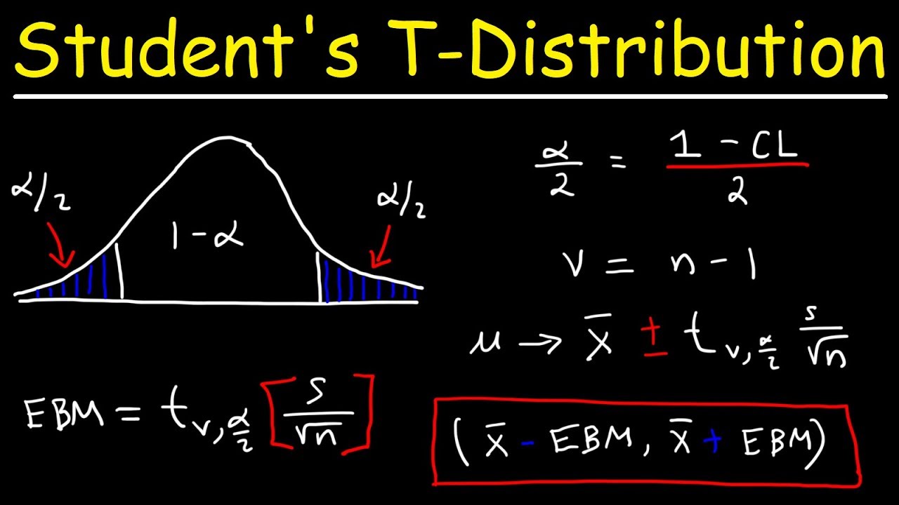
Confidence intervals for the mean are calculated using the t-distribution when the population standard deviation is unknown and the sample size is less than 30.

The critical values of T are found using calculators or distribution tables and denoted by T_sub_C.

Choosing between the T or Z distribution depends on the knowledge of the population standard deviation and the sample size.

The degree of freedom (DF) is calculated as the sample size minus one and is crucial for t-distribution calculations.

As sample size increases, the t-distribution approaches the Z-distribution.

A 95% confidence interval for the mean temperature of coffee from 16 randomly selected coffee shops is calculated.

The sample mean temperature is 162 Fahrenheit with a sample standard deviation of 10.

The t-distribution is used for constructing confidence intervals when the sample size is less than 30 and the population is approximately normally distributed.

The calculator automatically calculates the degree of freedom and provides the confidence interval.

For a 95% confidence interval, the mean temperature is estimated to be between 156.7 and 167.3 degrees Fahrenheit.

Estimating population proportions involves calculating P_hat and Q_hat from the sample data.

A survey example finds that 662 out of 1000 US adults find it acceptable to check personal emails at work.

The point of estimate for the population proportion is calculated as the number of successes divided by the sample size.

The margin of error for a confidence interval of a proportion is calculated using the formula involving P_hat, Q_hat, and the critical value Z.

A 95% confidence interval for the proportion of US teenagers who own smartphones is constructed using survey data.

The minimum sample size needed for a given confidence level and margin of error is calculated using a specific formula.

In political campaign scenarios, determining the minimum sample size is crucial for accurate estimation of voter preferences.

When no preliminary estimate is available, 0.5 is used for both P_hat and Q_hat in the sample size calculation formula.

A given P_hat of 0.31 requires calculating Q_hat as 0.69 to determine the minimum sample size for a political campaign.

The minimum sample size calculation must always be rounded up to ensure adequate representation.

Transcripts

Browse More Related Video

Student's T Distribution - Confidence Intervals & Margin of Error

Introduction to the t Distribution (non-technical)

Elementary Stats Lesson #16

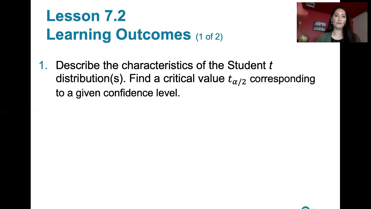
7.2.0 Estimating a Population Mean - Lesson Overview, Key Concepts, Learning Outcomes

Confidence Intervals | Population Mean: σ Unknown

7.2.1 Estimating a Population Mean - Student t Distribution and Finding Critical t Values

Related Tags

Confidence Intervals T-Distribution Sample Size Statistical Analysis Population Mean Standard Deviation Critical Value Data Interpretation Calculus Tools Estimation Methods Survey Analysis