Math 11 - Section 4.1
TLDRIn this engaging lecture, Professor Monti delves into the intriguing world of calculus, specifically focusing on the concept of antiderivatives. He begins by explaining the process of antidifferentiation, which involves finding the original function from its derivative. The professor then outlines the integral sign and its role in representing antiderivatives, emphasizing the inclusion of a constant (C) in the general antiderivative form. He proceeds to introduce several key rules and shortcuts for finding antiderivatives, such as the constant rule, power rule, and the natural logarithm rule. The lecture also highlights the importance of understanding the properties of integration, including the ability to separate integrals into sums or differences and the application of the constant multiple rule. Professor Monti reinforces the concepts with practical examples, demonstrating how to apply these rules to solve various integral problems. He further illustrates the process of finding functions with initial conditions, providing step-by-step solutions to real-world problems, such as determining demand functions from marginal demand. The lecture concludes with an invitation for students to ask questions and engage in further discussion, fostering a dynamic learning environment.
Takeaways
- 🔢 The process of finding antiderivatives is known as antidifferentiation, which is essentially reversing the process of taking derivatives to find the original function.
- ⚖️ The antiderivative of a function is represented by adding a constant (C) to the function, as it represents all possible antiderivatives of the given derivative.
- 📚 The integral sign (∫) is used to denote the antiderivative, and the integral of a function with respect to x is written as ∫f(x)dx.
- 🏎️ The power rule for antiderivatives states that the antiderivative of x^n is (x^(n+1))/(n+1) + C, where n is not equal to -1.
- 📈 The antiderivative of a constant times a function is the constant times the antiderivative of the function, following the constant multiple rule.
- ➕ The antiderivative of a sum or difference of functions can be found by finding the antiderivative of each function separately and then combining them.
- 🔁 The natural logarithm function, ln|x|, is the antiderivative of 1/x, accounting for the absolute value to include negative values of x.
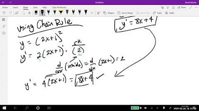
- 📌 The antiderivative of e^(ax) is (1/a)e^(ax) + C, which is derived from the chain rule in reverse when finding antiderivatives.
- 🔍 Checking the work by differentiating the found antiderivative to ensure it matches the original derivative function is a good practice to confirm accuracy.
- 📋 When provided with an initial condition, such as f(1) = 6, it is used to solve for the constant C in the antiderivative to find the specific function f(x).
- 🛒 Application problems, like finding a demand function from a marginal demand function, can be solved by antidifferentiation and applying initial conditions to find the specific function.
Q & A
What is the main topic of Chapter Four in the transcript?
-The main topic of Chapter Four is about finding antiderivatives, which is the process of going backwards from derivatives to find the original function.
What is the general form of the antiderivative of 3x?
-The general form of the antiderivative of 3x is 3x plus a constant C, where C can be any constant.
What is the antiderivative of a constant with respect to x?
-The antiderivative of a constant with respect to x is the constant times x plus another constant C.
What is the power rule for antiderivatives?
-The power rule for antiderivatives states that the antiderivative of x to the power of n is (x to the power of n+1) divided by (n+1) plus a constant C.
What is the antiderivative of the natural exponential function e^(ax) with respect to x?
-The antiderivative of e^(ax) with respect to x is (1/a) times e^(ax) plus a constant C.
How can you find the antiderivative of a sum or difference of functions?
-You can find the antiderivative of a sum or difference of functions by taking the antiderivative of each function separately and then adding or subtracting the results.
What is the process called when you find the original function from its derivative?
-The process is called antidifferentiation.
How can you check if your antiderivative is correct?
-You can check if your antiderivative is correct by taking the derivative of your antiderivative and verifying that it matches the original function.
What is the antiderivative of 1/x with respect to x?
-The antiderivative of 1/x with respect to x is the natural logarithm of the absolute value of x plus a constant C.
How does the constant multiple rule apply to antiderivatives?
-The constant multiple rule for antiderivatives allows you to factor out constants when taking the antiderivative of a function, and then multiply the result by the constant after the integration.
What is the process to find a function given its derivative and an initial condition?
-To find the original function given its derivative and an initial condition, you first find the antiderivative of the derivative, which gives you the general form of the function with an undetermined constant. Then, you use the initial condition to solve for this constant, thereby determining the specific function.
Outlines
📚 Introduction to Antiderivatives and Antidifferentiation
Professor Monti begins by introducing Chapter Four, which focuses on antiderivatives and the process of antidifferentiation. He explains that while derivatives give the rate of change, antiderivatives help find the original function. The concept is illustrated by showing that multiple functions can have the same derivative, such as 3x, 3x+7, and 3x-2, all of which are antiderivatives of 3. The integral sign is introduced as a notation for antiderivatives, and the general form of an antiderivative is expressed as a function plus a constant C.
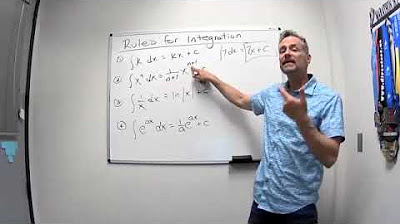
📝 Rules and Shortcuts for Antiderivatives
The video outlines several rules and shortcuts for finding antiderivatives. The first rule states that the antiderivative of a constant times a variable is the constant times the variable plus a constant C. The power rule is also discussed, where the antiderivative of x to the nth power is x to the power of n+1 divided by n+1, plus C. Additional rules cover the integration of a constant times a function and handling sums or differences by breaking them into separate integrals. Examples are provided to demonstrate the application of these rules.
🧮 Working Through Antiderivatives with Examples
The script continues with examples of calculating antiderivatives using the previously mentioned rules. It demonstrates the process of finding antiderivatives for expressions like x squared minus x plus two by breaking it down into individual parts and integrating each part separately. The process includes applying the power rule and combining results with a final constant C. The importance of checking the results by differentiating is emphasized for accuracy.
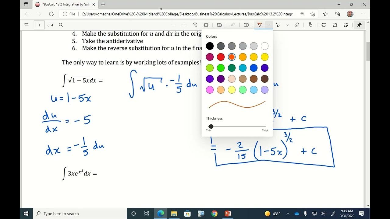
🔍 Applying Antiderivatives to More Complex Problems
The video script delves into more complex problems, such as integrating 1 over X to the fifth power and the third root of x squared. It shows how to rewrite expressions to fit the power rule and how to handle negative exponents. The script also addresses a common mistake with the natural logarithm function and its derivative, emphasizing the need to be cautious with constant multiples. Each step is detailed, and the process of integrating is shown to be systematic and straightforward once the rules are understood.
🧷 Finding Functions with Initial Conditions
The script explains how to find the original function when given the derivative and an initial condition. An example is provided where the derivative of a function is x minus 5, and it is known that the function equals 6 when x equals 1. By integrating the derivative and applying the initial condition, the constant C in the antiderivative is solved for, thus determining the original function. The process is checked by differentiating the found function to ensure it matches the given derivative and by plugging in the initial condition to verify the function's value.
🛒 Application of Antiderivatives in Demand Function
The final part of the script applies the concept of antiderivatives to find a demand function in economics. Given a marginal demand function, which is the derivative of the demand with respect to price, the demand function is found by antidifferentiating. An initial condition is provided to find the constant of integration. The script then shows how to use the demand function to find the quantity demanded at a specific price. This practical application demonstrates the utility of antiderivatives in real-world scenarios.
Mindmap
Keywords
💡Derivatives
💡Antiderivatives
💡Antidifferentiation
💡Integral Sign
💡Power Rule
💡Natural Logarithm
💡Exponential Function
💡Constant Multiple Rule
💡Sum and Difference Rule
💡Initial Conditions
💡Marginal Demand Function
Highlights
Introduction to Chapter Four, focusing on the concept of antiderivatives and the process of antidifferentiation.
Explanation of how to find the original function from its derivative by using antiderivatives.
General formula for the antiderivative of 3x, which includes an arbitrary constant C.
Use of the integral sign and the notation for the antiderivative of a function.
Listing of rules and shortcuts for finding antiderivatives, similar to those used in differentiation.
The power rule for antiderivatives, which involves adjusting the exponent and multiplying by the reciprocal.
The natural logarithm function as an antiderivative of 1/x, considering the absolute value of x.
The antiderivative of e^(ax) involves dividing by 'a', showcasing the reverse of the chain rule in differentiation.
Properties of integration that allow for the separation of integrals into sums or differences and the factorization of constants.
Verification of antiderivatives by differentiating the result to check if it matches the original function.
Example problem solutions demonstrating the application of antiderivatives and the use of initial conditions to find specific functions.
Technique to find the constant of integration 'C' by using an initial condition provided in a problem statement.
Application of antiderivatives in a real-world context, such as finding the demand function from a marginal demand function.
Use of initial conditions to determine the constant of integration and the original function in economic contexts.
Explanation of how to handle cases where the power rule does not apply directly, such as with 2/X.
Solution to an application problem involving the demand for flameless candles, showcasing the practical use of antiderivatives.
The importance of checking the solution by differentiating to ensure the derivative matches the given function and verifying initial conditions.
Encouragement for students to ask questions and engage in live sessions for further clarification.
Transcripts


5.0 / 5 (0 votes)
Thanks for rating: