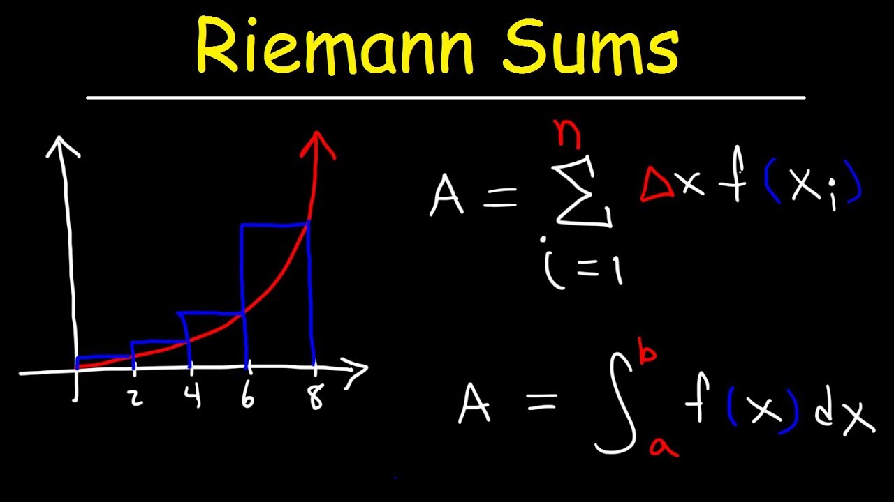
Riemann Sums - Midpoint, Left & Right Endpoints, Area, Definite Integral, Sigma Notation, Calculus

The Organic Chemistry Tutor

2 Nov 201668:07

EducationalLearning

32 Likes 10 Comments

TLDRThe video script focuses on various methods for calculating the area under a curve, such as using Riemann sums with left, right, and midpoint approximations, sigma notation, and limits. It demonstrates how to find the exact area by evaluating the definite integral and provides examples using different functions, such as x squared plus one and x cubed. The script also discusses the concepts of over and under approximations and how increasing the number of rectangles refines the accuracy of the approximations.

Takeaways

📊 The video demonstrates the process of finding the area under a curve using Riemann sums, including techniques utilizing left endpoints, midpoints, and right endpoints.
📝 It introduces the concept of sigma notation and limits as tools for calculating the area under a curve, enhancing understanding of mathematical notation.
📗 The definite integral is presented as a method to find the exact area under a curve, with a step-by-step guide on evaluating it for a given function.
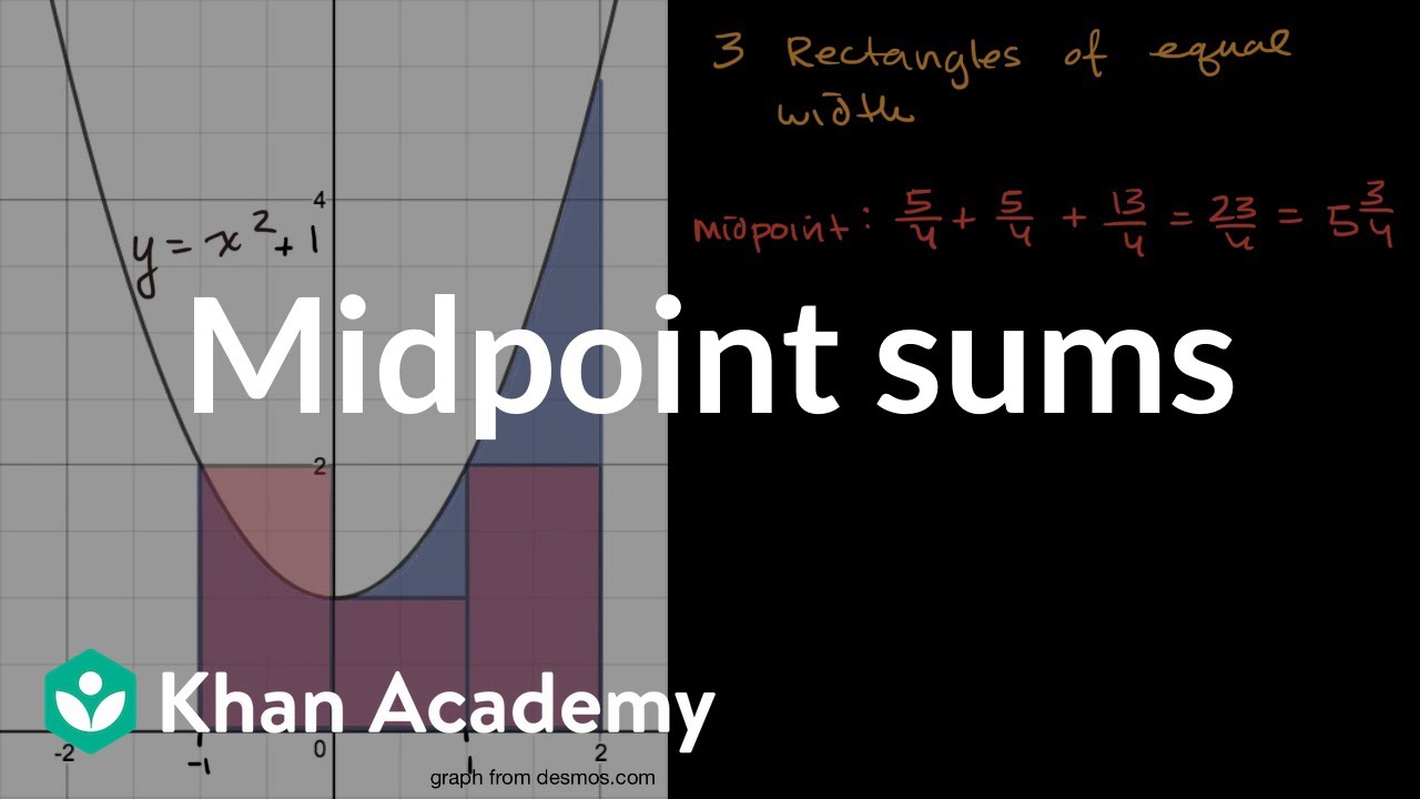
📈 A practical example is used to explain the calculation of area under the curve for the function f(x) = x^2 + 1, from x=0 to x=2, demonstrating the process in a clear, understandable manner.
📌 The video outlines the concept of delta x (Δx) as the width of rectangles in Riemann sums and how it affects the approximation of the area under the curve.
🔢 Utilizes a comparative approach to show how different methods (left endpoints, right endpoints, midpoint rule) provide different levels of approximation for the area under a curve.
🛠 Explains the significance of the number of rectangles (n) in Riemann sums and how increasing n leads to a more accurate approximation of the area under a curve.
💡 Offers insights into the conceptual understanding of underestimation and overestimation in the context of Riemann sums, particularly in relation to the function's behavior (increasing or decreasing).
🖥 Provides a comprehensive example using the function f(x) = x^3 to illustrate the application of Riemann sums and the definite integral for estimating areas.
📚 Discusses advanced topics such as the application of the antiderivative of 1/x, showcasing the calculation of areas with functions that have more complex antiderivatives.

Q & A

What is the fundamental concept behind finding the area under a curve in calculus?
-The fundamental concept involves calculating the definite integral of a function over a specific interval. This method provides the exact area under the curve from one point to another.
How can Riemann sums be used to approximate the area under a curve?
-Riemann sums approximate the area under a curve by dividing the area into small rectangles, calculating the area of each rectangle, and then summing these areas. This can be done using left endpoints, right endpoints, or midpoints of the rectangles.
What role does sigma notation play in calculating Riemann sums?
-Sigma notation is used to represent the sum of the areas of all rectangles in a Riemann sum. It provides a concise way to express the summation process, facilitating the calculation of the approximate area under the curve.
What is the significance of delta x in the context of Riemann sums?
-Delta x represents the width of each rectangle in a Riemann sum. It is calculated as the difference between the upper and lower bounds of the interval divided by the number of rectangles (n). Delta x is crucial for determining the size of each rectangle used in approximating the area under the curve.
How do left endpoints, midpoints, and right endpoints affect the approximation of an area under a curve?
-The choice of left endpoints, midpoints, or right endpoints affects the accuracy of the Riemann sum approximation. Left endpoints tend to underestimate, right endpoints overestimate, and midpoints provide a more balanced approximation for increasing functions. The opposite is true for decreasing functions.
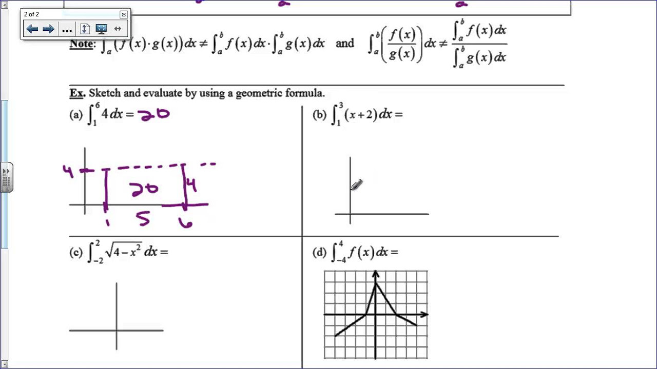
What is the anti-derivative and how is it used in finding the area under a curve?
-The anti-derivative of a function is another function whose derivative is the original function. In finding the area under a curve, the anti-derivative is used to calculate the definite integral, providing the exact area between the curve and the x-axis over a specified interval.
Why do the midpoint rule tend to provide a more accurate approximation compared to the left and right endpoint methods?
-The midpoint rule tends to be more accurate because it balances the overestimation and underestimation that can occur with the left and right endpoint methods, especially for curves that are not linear. The midpoints more closely represent the average value of the function over each subinterval.
What is the purpose of averaging the left and right endpoint Riemann sums?
-Averaging the left and right endpoint Riemann sums provides a better approximation of the area under the curve than either method alone. This average tends to be closer to the true area, especially when the function is either consistently increasing or decreasing.
How does increasing the number of rectangles (n) in a Riemann sum affect the approximation of the area under a curve?
-Increasing the number of rectangles (n) in a Riemann sum improves the accuracy of the area approximation. More rectangles mean smaller widths (delta x), which results in a better fit to the curve and a closer approximation to the actual area.
What is the relationship between the definite integral and the area under a curve?
-The definite integral of a function over an interval represents the exact area under the curve of the function between two points on the x-axis. It is the limit of the Riemann sums as the number of rectangles approaches infinity, providing the most accurate measurement of the area.

Outlines

00:00

📘 Introduction to Riemann Sums and Definite Integrals

This segment introduces the concept of finding the area under a curve using Riemann sums and the evaluation of definite integrals. It presents a detailed explanation of how to calculate the area under the curve for the function f(x) = x^2 + 1 from x=0 to x=2. The approach involves calculating the exact area by evaluating the definite integral of the function over the specified interval, followed by a step-by-step guide on how to perform this calculation, including finding the antiderivative and applying the evaluation theorem.

05:01

📏 Understanding Riemann Sums: Left, Right, and Midpoint Approaches

This section delves into the approximation of the area under a curve using Riemann sums, focusing on left endpoints, right endpoints, and midpoints. It provides a comprehensive explanation of how to calculate delta x (the width of each rectangle) and how to choose points for approximation using different endpoints. Furthermore, it contrasts the accuracy of these methods by comparing their approximations to the exact area, highlighting the underestimation or overestimation tendencies of each approach based on the function's behavior.

10:05

📊 Detailed Comparison and Graphical Representation of Riemann Sum Approaches

This paragraph compares the accuracy of different Riemann sum approaches (left endpoint, right endpoint, and midpoint) through numerical examples and explains the concepts of underestimation and overestimation. It introduces the strategy of averaging the left and right endpoint approximations for a potentially more accurate estimate. Additionally, it discusses the graphical representation of these methods, explaining how to draw rectangles for each approach and how these visualizations correlate with their respective underestimations or overestimations.

15:08

🔍 Exploring Riemann Sums with a New Function and Rectangle Count Variations

The narrative shifts to applying Riemann sum approximations to a new function, f(x) = x^3, over the interval from 0 to 4, using four rectangles. This section outlines the calculation of the exact area using the antiderivative and then explores the approximation of this area using left endpoints, right endpoints, and the midpoint rule. It illustrates how increasing the number of rectangles (n) improves the approximation accuracy, emphasizing the continuous effort to get closer to the exact area by adjusting the approximation method.

20:08

🔄 Averaging Endpoint Approximations and Introduction to Decreasing Functions

This part introduces the technique of averaging the left and right endpoint approximations as a method to closely approximate the actual area under a curve for an increasing function. It then transitions to examining the approximation of areas under a curve described by a decreasing function, specifically f(x) = 1/x, demonstrating how the tendencies of underestimation and overestimation shift when applying Riemann sum approximations to decreasing functions.

25:10

✏️ Deep Dive into Definite Integral Definitions and Calculations

The segment extends the discussion on Riemann sums and definite integrals by offering a detailed mathematical framework for understanding and applying these concepts to both increasing and decreasing functions. It elaborates on how to calculate areas using definite integrals and Riemann sums by introducing and utilizing formulas for x sub i, delta x, and sigma notation. The explanations include calculating areas using the right and left endpoints and illustrating how these calculations are affected by the function's direction of change.

30:10

🧮 Advanced Integral Calculations and Practical Examples

Focusing on advanced techniques for evaluating definite integrals and Riemann sums, this part introduces several key formulas for calculating the sum of sequences and applies these to practical examples. It provides a thorough explanation of how to use these formulas in the context of definite integrals, illustrating the process with examples that calculate areas under curves using sigma notation and limits. This detailed examination helps to demystify the complexities involved in approximating areas and evaluating integrals.

35:12

📚 Concluding with Complex Integral Evaluations and Applications

The final segment wraps up the discussion by applying the previously introduced mathematical principles and formulas to solve complex area problems using definite integrals. It showcases the practical application of these concepts through step-by-step examples, demonstrating how to evaluate areas under curves for various functions over specified intervals. This comprehensive overview highlights the utility and versatility of Riemann sums and definite integrals in solving real-world mathematical problems.

Mindmap

Keywords

💡Riemann sums

Riemann sums are a method for approximating the total area under a curve, which is a key concept in calculus and integral mathematics. This technique breaks down the area into a series of rectangles, and the sum of these rectangular areas approximates the area under the curve. In the video, Riemann sums are introduced as a means to estimate the area under a parabolic curve defined by the function f(x) = x^2 + 1, using left endpoints, midpoints, and right endpoints for the calculations. This method provides an intuitive approach to understanding definite integrals by visualizing and calculating areas incrementally.

💡Definite integral

The definite integral is a fundamental concept in calculus that represents the exact area under a curve between two points. It is calculated using the antiderivative of a function. In the script, the definite integral of the function f(x) = x^2 + 1 from 0 to 2 is evaluated to find the exact area under the curve, which contrasts with the approximate methods provided by Riemann sums. This illustrates how definite integrals provide precise results, serving as a cornerstone for understanding accumulation and area in calculus.

💡Sigma notation

Sigma notation, represented by the Greek letter sigma (Σ), is used to denote the sum of a series of terms. It simplifies the expression of adding many values together by indicating the starting point, ending point, and the formula for each term in the sequence. In the context of the video, sigma notation is used to express the sum of the areas of rectangles in Riemann sums, highlighting its utility in summarizing series and iterative calculations, particularly in the approximation of areas under curves.

💡Antiderivative

An antiderivative of a function is another function whose derivative is the original function. It is used to compute definite integrals, which represent the area under a curve. The video describes finding the antiderivative of f(x) = x^2 + 1 to evaluate the definite integral from 0 to 2. This concept is critical for understanding integration, as it provides the mathematical basis for finding areas under curves and solving differential equations.

💡Delta x (Δx)

Delta x (Δx) represents the width of each rectangle in Riemann sums. It is calculated as the difference between the upper and lower bounds of the interval divided by the number of rectangles (n). This term is essential for approximating the area under a curve using Riemann sums, as demonstrated in the video where Δx is used to calculate the width of rectangles that approximate the area under the curve f(x) = x^2 + 1. Δx allows for the division of the area into manageable segments for approximation.

💡Function

A function in mathematics is a relation that uniquely associates members of one set with members of another set. In the video, the function f(x) = x^2 + 1 is used as an example to illustrate the concept of finding areas under curves. The function, representing a parabola, serves as the basis for demonstrating Riemann sums, definite integrals, and the connection between antiderivatives and the calculation of areas, showcasing the practical applications of functions in calculus.

💡Midpoint rule

The midpoint rule is a technique for approximating the area under a curve by using the midpoint of the top of each rectangle to estimate the height. It is one of the methods for calculating Riemann sums. In the video, the midpoint rule is employed to approximate the area under f(x) = x^2 + 1, highlighting its accuracy compared to using left or right endpoints. This rule often yields a more precise approximation of the integral, as it balances the overestimation and underestimation of the curve by the rectangles.

💡Approximation

Approximation in the context of the video refers to the process of estimating the area under a curve using methods that provide close but not exact values, such as Riemann sums. Different approaches, including using left endpoints, midpoints, and right endpoints, offer various degrees of accuracy. The concept is crucial for understanding how mathematicians and scientists can apply calculus to real-world situations where exact solutions are not feasible, demonstrating the practical value of approximation techniques in analysis.

💡Interval

An interval refers to the range between two points on the number line, often representing the domain or portion of a graph over which calculations are performed. In the video, the interval from 0 to 2 is used as the domain for finding the area under the function f(x) = x^2 + 1. Intervals are fundamental in calculus for defining the limits of integration and the segments over which Riemann sums are calculated, emphasizing their role in delineating the scope of mathematical analysis.

💡Sigma notation

Sigma notation, represented by the Greek letter sigma (Σ), is used to denote the sum of a series of terms. It simplifies the expression of adding many values together by indicating the starting point, ending point, and the formula for each term in the sequence. In the context of the video, sigma notation is used to express the sum of the areas of rectangles in Riemann sums, highlighting its utility in summarizing series and iterative calculations, particularly in the approximation of areas under curves.

Highlights

Introduction to finding the area under a curve using Riemann sums and definite integrals.

Explanation of the definite integral as a method to find the exact area under a curve.

Deriving the anti-derivative of x squared plus one and calculating its definite integral.

Overview of Riemann sums and the concept of approximating area under a curve using rectangles.

Explanation of left, right, and midpoint Riemann sums for area approximation.

Calculation of area under the curve using left endpoint Riemann sums.

Demonstration of midpoint Riemann sums for more accurate area approximation.

Comparison of left, midpoint, and right Riemann sums for accuracy in area estimation.

Graphical representation of Riemann sums and their relation to the curve.

Illustration of how increasing the number of rectangles improves Riemann sum accuracy.

Introduction to anti-derivatives and the calculation of definite integrals.

Example of calculating area using definite integrals with different functions.

Application of the sigma notation and limits to define the definite integral.

Exploration of the relationship between function behavior (increasing or decreasing) and the accuracy of Riemann sum approximations.

Use of mathematical formulas and limits to simplify and evaluate definite integrals.

Transcripts

Browse More Related Video

Riemann Sums - Left Endpoints and Right Endpoints

Riemann Sums

Integration and Area under a Curve

Riemann Sums and Definite Integrals

Midpoint sums | Accumulation and Riemann sums | AP Calculus AB | Khan Academy

BusCalc 13.4 Riemann Sums

Related Tags

Mathematics Calculus Integrals Riemann Sums Area Calculation Left Endpoints Midpoint Rule Right Endpoints Antiderivative Limits