BusCalc 13.4 Riemann Sums
TLDRThe transcript details a comprehensive lesson on calculus, specifically focusing on integration by parts and the concept of Riemann sums. The instructor begins by guiding through the process of finding anti-derivatives using integration by parts, illustrating the method with examples involving functions like x^3 and e^(2x). The lesson then transitions into the application of Riemann sums for approximating the area under a curve, which is not a standard shape like a circle, triangle, or rectangle. The Riemann sum technique involves dividing the area under the curve into rectangles and summing their areas. As the number of rectangles (n) increases, the approximation error decreases, with the limit as n approaches infinity providing the exact area under the curve, known as the definite integral. The instructor also discusses the use of calculators for numerical integration, which employs Riemann sums with a high number of rectangles for increased accuracy. The summary concludes with the importance of understanding the manual calculation process to grasp how computers and calculators perform these calculations.
Takeaways
- 📚 The concept of anti-derivatives is introduced through integration by parts, a method for integrating complex functions by breaking them down into simpler components.
- ✅ The constant factor of an integral can be pulled out of the integrand, which is a property useful for both derivatives and anti-derivatives.
- 🔢 Integration by parts involves setting up a table to determine the derivatives and anti-derivatives of the functions involved, which is key to solving the integral.
- 📈 The antiderivative of e^{2x} is \( \frac{1}{2}e^{2x} \), which is a rule that students are expected to memorize from their notes.
- 🔑 When integrating functions involving natural logarithms, it's important to place the natural logarithm in the first column of the integration by parts table to avoid having to find the anti-derivative of the natural logarithm.
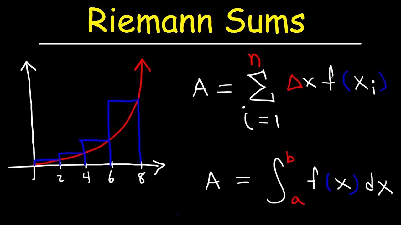
- 📉 The Riemann sums are introduced as a method for calculating the areas of irregular shapes by approximating them with a series of rectangles.
- 🔍 As the number of rectangles (n) used in the Riemann sum increases, the relative error decreases, leading to a more accurate approximation of the area under the curve.
- 📏 The width of each rectangle in a Riemann sum is determined by dividing the interval length (b - a) by the number of rectangles (n).
- 📐 The height of each rectangle is determined by the function's value at specific points along the x-axis, which corresponds to the left side of each rectangle.
- 🧮 The summation notation (∑) is used to represent the addition of all the areas of the rectangles in the Riemann sum, which is an approximation of the area under the curve.
- 🎓 The definite integral is the exact area under the curve, which is found by taking the limit of the Riemann sum as n approaches infinity or as the width of each rectangle (Δx) approaches zero.
- 📊 Calculators and computers use numerical integration techniques, which are essentially refined Riemann sums with a very high number of rectangles, to find the area under a curve.
Q & A
What is the main topic discussed in the first part of the transcript?
-The main topic discussed in the first part of the transcript is the process of finding anti-derivatives using integration by parts, with a focus on two specific questions involving this technique.
How does the speaker simplify the integration of 4x^3 * e^(2x)?
-The speaker simplifies the integration by first taking the constant factor '4' out of the integrand. Then, using a table for integration by parts, the speaker identifies x^3 and e^(2x) for the integration, taking derivatives and anti-derivatives accordingly, and finally combining the results to find the anti-derivative.
What is the antiderivative rule mentioned for e^(2x)?
-The antiderivative rule mentioned for e^(2x) is that the antiderivative of e^(2x) is (1/2)e^(2x), which comes from the rule set in section 13.1 of the speaker's notes.
What is the strategy for the integration by parts when there is a natural log function involved?
-When there is a natural log function involved in an integration by parts, the speaker suggests that you only need two rows in your integration by parts table. The natural log part should always be in the first column, and you can stop after the second row because the anti-derivative of natural log does not simplify further.
What is the main idea behind Riemann sums?
-The main idea behind Riemann sums is to calculate the areas of shapes that are not regular polygons, such as circles, triangles, or rectangles. This is done by dividing the area under a curve into rectangles and summing their areas to approximate the total area under the curve.
How does the number of rectangles (n) affect the accuracy of the Riemann sum approximation?
-As the number of rectangles (n) increases, the width of each rectangle (delta x) decreases, leading to a more precise approximation of the area under the curve. The relative error approaches zero as n approaches infinity, making the estimate very close to the actual area.
What is the formula for the height of the j-th rectangle in a Riemann sum?
-The height of the j-th rectangle in a Riemann sum is given by the function evaluated at the point a plus (j-1) times the width of each rectangle, which is f(a + (j-1) * (b-a)/n).
How does the speaker describe the process of numerical integration on a calculator?
-The speaker describes the process of numerical integration on a calculator as using a Riemann sum algorithm. The calculator starts with a certain number of rectangles, calculates the area, and then increases the number of rectangles in iterative steps, refining the answer until the Riemann sums do not change significantly, at which point it provides the estimated area.
What is the significance of the limit notation in the context of definite integrals?
-The limit notation is used to express the concept that as the number of rectangles (n) approaches infinity, or equivalently, as the width of each rectangle (delta x) approaches zero, the Riemann sum approaches the actual area under the curve. This limit process defines the definite integral.
How does the speaker use Desmos to demonstrate the concept of Riemann sums?
-The speaker uses Desmos to create graphics that visually represent the area under a curve being divided into rectangles of varying widths. By adjusting the number of rectangles, the speaker shows how the approximation of the area changes and how it converges to the actual area as the number of rectangles increases.
What is the practical application of understanding Riemann sums and definite integrals?
-Understanding Riemann sums and definite integrals is important because it provides insight into how calculators and computers perform numerical integration and area calculations under curves. This knowledge helps users to not be merely users of technology but to understand the underlying mathematical processes.
Outlines
📚 Integration by Parts and Anti-Derivatives
The paragraph begins with an introduction to solving integration problems using the method of integration by parts, a technique previously discussed. The speaker simplifies the problem by taking the constant factor 'four' out of the integrand, which is permissible when dealing with derivatives or anti-derivatives. A table is constructed to apply the integration by parts formula, with the left column representing the function of x cubed and the right column representing the exponential function e to the 2x. The derivatives and anti-derivatives of these functions are calculated, leading to a final expression for the anti-derivative of the given function, which includes a constant of integration 'c'. The paragraph concludes with an invitation for questions, transitioning into the next problem involving finding the anti-derivative of a different function.
🧮 Applying Integration by Parts to Natural Logs
The second paragraph focuses on applying integration by parts to a function involving a natural logarithm. The speaker outlines the process of setting up the integration by parts formula with 'natural log of t' and 't squared' as the initial functions. The derivatives and anti-derivatives are calculated, leading to a step involving the anti-derivative of a horizontal grouping. The process concludes with the addition of a constant 'c'. It is highlighted that when dealing with natural logs in integration by parts, only two rows are needed in the table, and the natural log should always be placed in the first column to avoid needing to find the anti-derivative of the natural log itself. The paragraph ends with a teaser for the next topic: Riemann sums.
📏 Riemann Sums and Calculating Irregular Shapes
The third paragraph introduces Riemann sums as a method for calculating the areas of irregular shapes that cannot be broken down into simple geometric shapes like triangles or rectangles. The process involves dividing the area under the curve into 'n' rectangles and using the function's value at the left side of each rectangle as the height. The area of each rectangle is calculated and then summed to estimate the total area under the curve. The concept of relative error is discussed, showing how it decreases as the number of rectangles increases, providing a more accurate estimate. The actual area under the curve is revealed to be 5.39, and the process is demonstrated with a step-by-step calculation using three and then eight rectangles to illustrate the decreasing error.
📈 Increasing Accuracy with More Rectangles
The fourth paragraph delves deeper into the concept of using more rectangles to decrease the relative error and approximate the area under a curve more closely. It is shown that with 20 rectangles, the error is about two percent, and with 30 rectangles, it drops to 2.5 percent. The speaker uses Desmos to create graphics for visual aid and explains how the choice of the function and the number of rectangles can affect the error. The paragraph concludes with a table summarizing that as the number of rectangles increases, the relative error approaches zero, and the estimate using the areas of the rectangles approaches the actual area of the shape.
🔢 Calculating Rectangle Widths and Riemann Sums
The fifth paragraph explains the algebraic process of calculating the width of each rectangle used in the Riemann sum and how to express the height of each rectangle in terms of the function evaluated at specific points. The width of each rectangle is determined by dividing the interval length (b - a) by the number of rectangles (n). The height of each rectangle is the function evaluated at points a + (j - 1) * (b - a) / n, where j is the rectangle number. The paragraph introduces summation notation and explains how to sum the areas of all rectangles to approximate the area under the curve. It concludes with a discussion of how different notations can be used to represent the same mathematical concept.
🎓 Understanding Riemann Sums and Definite Integrals
The sixth paragraph continues the discussion on Riemann sums and introduces definite integrals as the exact area under a curve, which is found by taking the limit as the number of rectangles (n) approaches infinity and the width of each rectangle (delta x) approaches zero. The paragraph explains that as the number of rectangles increases, the error decreases, and the approximation gets closer to the actual area. It also touches on the use of different notations, such as the integral symbol with limits, to represent the process of finding the area under a curve. The concept of a microscopic change in the x variable (dx) is introduced, which is used when the change is so small that it's not observable, akin to the deltas used in derivatives.
📊 Numerical Integration and Calculator Usage
The seventh paragraph discusses how calculators use the concept of Riemann sums to perform numerical integration and find the area under a curve. The speaker demonstrates how to use a calculator to find the area under a parabola defined by the function half x squared plus one, between the bounds of zero and one. The calculator's process is described as incrementally increasing the number of rectangles used in the Riemann sum until the change between successive approximations is minimal, indicating a sufficiently accurate result. The paragraph emphasizes that the calculator's numerical integration feature uses an algorithm that adds up the areas of many small rectangles to approximate the integral.
📉 Estimating Areas with Different Numbers of Rectangles
The eighth paragraph illustrates the process of estimating the area under a curve using different numbers of rectangles. The focus is on a parabola represented by the function x squared plus one, with the interval from 0 to 3. The speaker shows how to calculate the area using two, four, and eight rectangles, providing detailed steps for each case. The heights of the rectangles are determined by evaluating the function at specific points, and the areas are calculated by multiplying the heights by the width of the rectangles. The results from using different numbers of rectangles are compared, showing how the approximation improves with more rectangles.
🔍 Refining the Approximation with More Rectangles
The ninth paragraph continues the process of refining the area approximation under a curve by increasing the number of rectangles to eight. The speaker calculates the height of each rectangle by evaluating the function at the left side of each rectangle and then multiplies the sum of these heights by the width of the rectangles to find the area. The process is shown to be iterative, with the speaker using a calculator to find the necessary function evaluations. The paragraph emphasizes the importance of order of operations and the use of parentheses in calculations, especially when using a calculator.
📝 Understanding the Calculation Process and Technology
The final paragraph summarizes the process of calculating areas under a curve using Riemann sums and highlights the importance of understanding the underlying method, even though it may be tedious. The speaker relates the process to the functioning of calculators and computers, which perform similar calculations more efficiently. The paragraph concludes with a note on the use of numerical integration on calculators to find areas under curves and an encouragement for students to practice the method before an upcoming exam.
Mindmap
Keywords
💡Anti-derivative
💡Integration by parts
💡Derivatives
💡Riemann sums
💡Relative error
💡Definite integral
💡Numerical integration
💡Limit notation
💡Curvy shapes
💡Error estimation
💡Desmos
Highlights
Integration by parts is used to find anti-derivatives, as demonstrated with the given examples.
Constants can be factored out of integrals, a property useful for both derivatives and anti-derivatives.
The process of filling out an integration by parts table is explained, including the selection of functions for the integral and their derivatives.
The antiderivative of e^(ax) is a memorized rule where the exponential function remains the same but is divided by the constant inside the exponent.
The concept of stopping the integration by parts process after a certain number of terms is discussed, particularly when dealing with functions that never reach zero.
The second question involves a different function and a reminder that integration by parts can be used for a variety of functions, not just exponentials.
Natural log functions in integration by parts require only two rows in the table, and the process is explained up to the antiderivative of t^2.
Riemann sums are introduced as a method to calculate areas of irregular shapes that are not easily defined by standard geometric formulas.
A five-step procedure for using Riemann sums to estimate areas under a curve is outlined.
The relationship between the number of rectangles used in a Riemann sum and the accuracy of the area approximation is discussed.
Desmos is mentioned as a tool for visually demonstrating the process of approximating areas using Riemann sums.
The concept of relative error in approximations is explained, and how it decreases as the number of rectangles increases.
The formula for the height of a rectangle in a Riemann sum is detailed, including the use of function evaluation at specific points.
The summation notation is introduced to represent the addition of areas of multiple rectangles in a Riemann sum.
The use of limit notation to describe the area under a curve as the number of rectangles approaches infinity is explained.
The connection between the width of rectangles (delta x) and the number of rectangles (n) is discussed in the context of refining approximations.
The transition from Riemann sums to definite integrals is described, emphasizing the limit as delta x approaches zero.
The concept of dx representing an infinitesimally small change in x is introduced, relating to the idea of derivatives in calculus.
Numerical integration on calculators is shown to be a practical application of Riemann sums, using a large number of rectangles for precise area calculation.
The importance of understanding the manual calculation of Riemann sums is emphasized for a deeper comprehension of calculator and computer calculations.
Transcripts
Browse More Related Video
Riemann Sums - Left Endpoints and Right Endpoints

What Is an Integral?
Riemann Sums and Definite Integrals
Writing an Integral as a Limit of a Riemann Sum

AP Calculus AB: Lesson 6.2 Part 2 (Limit Definition of Definite Integral)
Definite integral as the limit of a Riemann sum | AP Calculus AB | Khan Academy
5.0 / 5 (0 votes)
Thanks for rating: