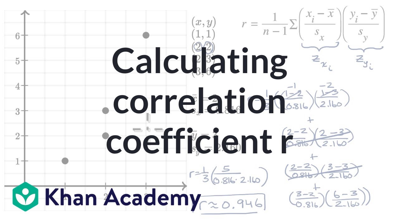
How To Calculate The Covariance Between X and Y - Statistics
TLDRThis video explains how to calculate the covariance between two variables X and Y, using a formula that involves finding the differences between each X and Y value and their respective means. It then walks through two example data sets, showing how to organize the data in a table to plug into the formula. The resulting positive and negative covariance values correspond to the positive and linear relationships graphed for each data set. Covariance indicates the direction of the relationship between variables.
Takeaways
- 📝 The covariance between two variables X and Y is calculated using the sum of the products of the differences between each X (or Y) value and their respective means, divided by N-1 for sample covariance or N for population covariance.
- 📈 Sample covariance is used in the example, emphasizing the formula's adjustment to N-1 to account for sample size.
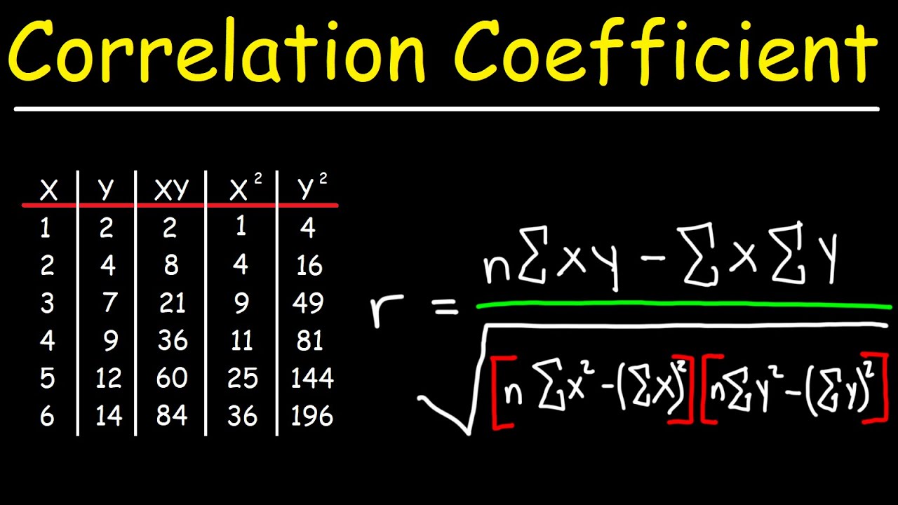
- 📚 A step-by-step approach involves creating a table with columns for X values, Y values, their differences from their means, and the products of these differences.
- 📲 The script demonstrates the process with a detailed example, including calculating means (×ar and Y×ar) and differences from the means.
- 🔧 The sum of the products column is crucial for calculating covariance, illustrating the interaction between X and Y's deviations from their means.
- 📉 Two example problems are solved to show both positive and negative covariance, indicating different types of relationships between variables.
- 📱 Covariance is positive when as one variable increases, the other also increases, suggesting a direct relationship.
- 💧 Negative covariance occurs when an increase in one variable corresponds with a decrease in the other, indicating an inverse relationship.
- 📖 If the covariance is zero, it suggests no linear relationship between X and Y.
- 📺 The explanation includes plotting the data points on graphs to visually demonstrate the linear relationships and the significance of positive or negative covariance.
Q & A
What is the formula used to calculate covariance between two variables X and Y?
-The formula is: Σ(X - X̅) * (Y - Ȳ) / (n - 1), where X̅ is the mean of X, Ȳ is the mean of Y, and n is the sample size.
Why do we use n-1 in the denominator for sample covariance?
-Using n-1 in the denominator adjusts for bias in estimating the population variance from a sample. This gives an unbiased estimator of the population covariance.
What does a positive covariance value indicate about the relationship between two variables?
-A positive covariance indicates that as one variable increases, the other variable also tends to increase, so there is a positive linear relationship between the variables.
What does a negative covariance value indicate?
-A negative covariance value indicates an inverse linear relationship - as one variable increases, the other tends to decrease.
What do the difference columns (X - X̅) and (Y - Ȳ) represent in the covariance formula?
-These difference columns represent the deviation of each data point from the mean. Taking these deviations allows us to measure how X and Y vary in relation to their means.
Why is the sum of the (X - X̅) column and (Y - Ȳ) column equal to zero?
-This is because the deviations sum to zero when calculated from the mean. The mean balances out positive and negative deviations.
What happens if the covariance between two variables equals zero?
-A covariance of zero indicates the variables are independent - there is no linear relationship between them.
How can you visually determine if two variables have positive or negative covariance based on their scatter plot?
-If high (low) values of one variable tend to occur with high (low) values of the other, the variables have positive covariance and an upwards sloping scatter plot. If highs occur with lows, there is negative covariance and a downwards sloping relationship.
What are some applications of covariance?
-Covariance is used in statistics and machine learning for understanding relationships between variables during regression analysis, financial modeling, pattern recognition, and more.
What happens to covariance if you standardize the variables before analysis?
-Standardizing gives variables a mean of 0 and standard deviation of 1. This results in the covariance becoming equal to the correlation coefficient between the standardized variables.
Outlines
😀 Introduction to Covariance
This paragraph introduces the topic of covariance. It explains that we will learn how to calculate the covariance between two variables X and Y using a specific equation. The paragraph also notes that the sample covariance uses n-1 in the denominator while population covariance uses just n.
😃 Calculating Covariance Using a Table
This paragraph demonstrates how to calculate covariance using a table. It shows how to organize the data into columns for X, Y, X-Xbar, Y-Ybar, and (X-Xbar)*(Y-Ybar). It then calculates the means Xbar and Ybar, fills out the table, sums the final column, and plugs the values into the covariance formula.
😊 Second Example Problem for Covariance
This paragraph works through a second example problem to calculate covariance between two variables X and Y, again using a table to organize the steps. It shows how to calculate the means, differences from the means, products of the differences, sum the products, and ultimately calculate the covariance.
😎 Interpreting Covariance from Graphs
This final paragraph relates covariance to visual relationships between variables on graphs. It shows two graphs with positive and negative slopes, relating them to the positive and negative covariances calculated in the examples. It explains covariance indicates the direction of the linear relationship between variables.
Mindmap
Keywords
💡Covariance
💡Sample Covariance
💡Population Variance
💡Mean
💡Differences from the Mean
💡Product of Differences
💡Linear Relationship
💡Positive Covariance
💡Negative Covariance
💡Graphical Representation
Highlights
The speaker discusses using computational modeling to understand how the brain encodes memories.
They developed a hippocampal model that can store memories in a compressed way similar to the brain.
The model exhibits replay of memories during rest periods, supporting theories about memory consolidation.
They found neural structure emerges in the model that matches anatomy of the hippocampus.
The speaker explains how they validated their model by comparing to recordings of neuron activity in rats.
They demonstrated the model can complete patterns from degraded inputs, like the brain does.
The model provides a new theoretical framework for episodic memory based on efficient coding principles.
The speaker speculates these coding strategies may facilitate memory retrieval and imagined simulations.
They are working to scale up the model to capture more complex memories and knowledge.
The model makes predictions about memory deficits that can be tested experimentally.
This modeling approach will advance understanding of memory disorders like amnesia and Alzheimer's disease.
The speaker concludes that brain-inspired AI can shed light on core neuroscience questions.
They are building virtual hippocampi to test theories of memory function that are difficult to probe in the brain.
The speaker emphasizes collaboration between neuroscience and AI can accelerate progress in both fields.
They propose using AI models as theoretical frameworks to guide and interpret neuroscience experiments.
Transcripts
Browse More Related Video


5.0 / 5 (0 votes)
Thanks for rating: