Integration and Area under a Curve

Chad Gilliland

30 Oct 201315:21

EducationalLearning

32 Likes 10 Comments

TLDRThis script explores various methods for estimating the area under a graph, using a car's speed over time as an example. It introduces the concept of Riemann sums, named after the German mathematician Bernhard Riemann, and demonstrates three techniques: left Riemann sums, right Riemann sums, and midpoint Riemann sums. The script provides a step-by-step guide on how to calculate these sums using rectangles based on different endpoints or midpoints of intervals, illustrating the process with a graph of speed over time and a function y = x^2 + 1.

Takeaways

📊 The video discusses estimating the area under a graph, specifically using a car's speed over time as an example of a monotonically increasing function.
📈 The script introduces the concept of Riemann sums, named after German mathematician Bernhard Riemann, as a method to calculate the area under a curve.
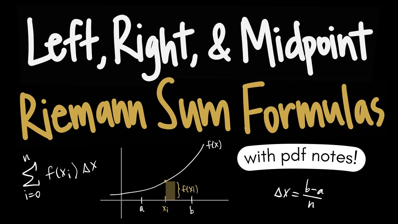
📚 Three types of Riemann sums are explained: left Riemann sums, right Riemann sums, and midpoint Riemann sums, each using different endpoints to estimate the area.
📐 The left Riemann sum uses the left endpoint of each interval to calculate the area of rectangles that approximate the area under the curve.
📏 The right Riemann sum uses the right endpoint of each interval for the same purpose, providing a different approximation of the area.
🎯 The midpoint Riemann sum uses the midpoint of each interval to find a more accurate approximation of the area under the curve.
📝 The script provides a step-by-step guide on how to calculate each type of Riemann sum, including the formula for the width of rectangles (Δx = (b - a) / n).
🛣️ The area under the speed graph of a car can be interpreted as the total distance traveled, which is why the units 'feet per second' are used in the example.
📉 The script also covers an example with the function y = x^2 + 1 to demonstrate how to estimate the area under a curve using a left Riemann sum with four equal subintervals.
👨‍🏫 The video is educational, aiming to teach viewers how to estimate areas under graphs using Riemann sums, with a focus on clarity and step-by-step instruction.
👋 The presenter ends the video with a light-hearted reminder for viewers to express love to their family members, adding a personal touch to the educational content.

Q & A

What is the main topic discussed in the video?
-The main topic discussed in the video is the method of estimating the area under a graph, specifically using Riemann sums.
What is a monotonically increasing function?
-A monotonically increasing function is a function that either always increases or remains constant, but never decreases.
What is the significance of the graph in the video?
-The graph in the video represents the speed of a car over a 12-second interval, with the x-axis labeled as time and the y-axis as speed in feet per second.
What is a Riemann sum and why is it used?
-A Riemann sum is a method used to approximate the area under a curve by dividing the area into rectangles and summing their areas. It was developed by German mathematician Bernhard Riemann.
What are the different types of Riemann sums mentioned in the video?
-The video mentions three types of Riemann sums: left Riemann sum, right Riemann sum, and midpoint Riemann sum.
How is the left Riemann sum calculated?
-The left Riemann sum is calculated by using the left endpoint of each subinterval to determine the height of the rectangles and multiplying it by the width of each rectangle.
How is the right Riemann sum calculated?
-The right Riemann sum is calculated by using the right endpoint of each subinterval to determine the height of the rectangles and multiplying it by the width of each rectangle.
What is the midpoint Riemann sum and how is it different from the other Riemann sums?
-The midpoint Riemann sum uses the midpoint of each subinterval to determine the height of the rectangles. It is different from the left and right Riemann sums because it uses the midpoint values instead of the endpoints.
What is the formula for calculating the width of each rectangle in a Riemann sum?
-The formula for calculating the width of each rectangle in a Riemann sum is Δx = (b - a) / n, where a and b are the endpoints of the interval and n is the number of subintervals.
How does the area under the curve of a speed graph relate to the total distance traveled?
-The area under the curve of a speed graph represents the total distance traveled because the area is calculated by multiplying the time (width of the rectangle) by the speed (height of the rectangle), resulting in distance.

Outlines

00:00

📈 Introduction to Estimating Area Under a Graph Using Riemann Sums

The script introduces the concept of estimating the area under a graph, specifically using a car's speed over time as an example. The car's speed is represented as a monotonically increasing function over a 12-second interval. The instructor explains the process of using Riemann sums to estimate this area, starting with a left Riemann sum, which involves drawing rectangles at the height of the left endpoints of the intervals. The method is demonstrated with a step-by-step guide on how to calculate the area of each rectangle and the total distance traveled by the car, which corresponds to the area under the speed graph.

05:01

📚 Exploring Different Riemann Sum Techniques

This paragraph delves deeper into the Riemann sum technique, contrasting the left Riemann sum with the right Riemann sum and the midpoint Riemann sum. The right Riemann sum is explained by drawing rectangles using the right endpoints of the intervals, while the midpoint Riemann sum involves calculating the height of rectangles at the midpoint of each interval. The script provides a practical example of estimating the area under the curve of the function y = x^2 + 1 from 0 to 2, using the left Riemann sum with four equal subintervals, and explains the formula for calculating the width of each rectangle (Delta X).

10:04

📝 Applying Riemann Sums to a Specific Function

The script continues with a detailed application of the Riemann sum technique to the function y = x^2 + 1, calculating the area from 0 to 2 using both left and right Riemann sums. The left Riemann sum is calculated by plugging in the left endpoint values of the intervals into the function and multiplying by the width of the rectangles. Similarly, the right Riemann sum is performed using the right endpoint values. The process is illustrated with clear instructions on how to find the height of each rectangle and how to perform the calculations, emphasizing the visual aspect of the rectangles on the graph.

15:07

🔍 Completing the Riemann Sum with Midpoint Estimation

The final paragraph concludes the lesson on Riemann sums by introducing the midpoint Riemann sum for the function y = x^2 + 1. The midpoint sum involves finding the midpoint of each interval and using the function's value at these points to determine the height of the rectangles. The script outlines the steps to calculate the area under the curve using this method, providing a comprehensive overview of how to find the midpoints, calculate the corresponding function values, and sum up the areas of the rectangles to estimate the total area under the curve.

Mindmap

Keywords

💡Estimating Area

Estimating area in the context of the video refers to calculating the area under a graph, which represents a function, using different methods. The main theme of the video is to teach viewers how to estimate this area, particularly for a graph representing a car's speed over time. The script discusses using Riemann sums to approximate the area under the curve, which is a fundamental concept in calculus.

💡Graph

A graph in the video is a visual representation of data points on a coordinate plane, with the x-axis typically representing time and the y-axis representing speed in feet per second. The script describes a graph of a car's speed over a 12-second interval, which is monotonically increasing, meaning it only goes up and does not decrease.

💡Riemann Sum

A Riemann sum is a method used in calculus to approximate the definite integral of a function. In the video, it is the central technique for estimating the area under the graph of the car's speed. The script explains different types of Riemann sums, such as left Riemann sum, right Riemann sum, and midpoint Riemann sum, each using different endpoints to estimate the area.

💡Monotonically Increasing Function

A monotonically increasing function is one where the function values increase as the independent variable (in this case, time) increases. The video uses this concept to describe the car's speed function, which never decreases over the 12-second interval, making it a suitable candidate for the area estimation methods discussed.

💡Left Riemann Sum

The left Riemann sum is a specific method of approximating the area under a graph where rectangles are drawn using the left endpoint of each interval. The script demonstrates this by drawing rectangles from time 0 to 3 seconds, 3 to 6 seconds, and so on, using the speed value at the beginning of each interval as the height of the rectangle.

💡Right Riemann Sum

In contrast to the left Riemann sum, the right Riemann sum uses the right endpoint of each interval to determine the height of the rectangles. The script illustrates this by drawing rectangles with heights corresponding to the speed values at the end of each interval, such as 37, 45, 54, and 65 feet per second.

💡Midpoint Riemann Sum

The midpoint Riemann sum is another method where the height of the rectangles is determined by the value of the function at the midpoint of each interval. The script explains this by finding the midpoint between the endpoints, such as between 0 and 6 seconds, and using the function value at that midpoint as the height for the rectangle.

💡Rectangles

In the context of the video, rectangles are used to approximate the area under the graph. The script describes drawing rectangles with varying widths and heights to represent the area under different parts of the graph, using the left, right, or midpoint values of the function to determine the height of each rectangle.

💡Endpoints

Endpoints in the video refer to the starting and ending points of each interval on the x-axis of the graph. The script uses the terms 'left endpoint' and 'right endpoint' to describe where the rectangles are drawn for the Riemann sums, with the left endpoint being the starting point and the right endpoint being the ending point of the interval.

💡Midpoint

The midpoint in the video is the exact middle point between two endpoints of an interval. The script explains how to find the midpoint for the midpoint Riemann sum by taking the average of the left and right endpoints, which is then used to determine the height of the rectangle for that interval.

💡Delta X

Delta X, often denoted as Δx, is the width of each rectangle in the Riemann sum approximation. The script mentions a formula for calculating Δx as the difference between the upper limit (B) and lower limit (a) of the interval divided by the number of subintervals (n), which is essential for setting up the Riemann sums.

Highlights

Introduction to estimating the area under a graph using Riemann sums.

Explanation of a monotonically increasing function with a car's speed as an example.

Visual representation of the function through a possible graph.

Introduction to the concept of Riemann sums with a historical note on George Bernard Riemann.

Demonstration of calculating a left Riemann sum using the left endpoints of intervals.

Step-by-step construction of rectangles for the left Riemann sum to estimate area.

Interpretation of the area under the curve as the total distance traveled.

Calculation of the left Riemann sum using specific speed values and time intervals.

Introduction to the right Riemann sum using right endpoints instead of left.

Construction of rectangles for the right Riemann sum with a new graph illustration.

Calculation of the right Riemann sum with the areas determined by right endpoint function values.

Introduction to the midpoint Riemann sum with a focus on midpoints of intervals.

Explanation of the midpoint Riemann sum process with a graph example.

Calculation of the midpoint Riemann sum using midpoint function values.

Application of Riemann sums to the function y = x^2 + 1 for estimating area from 0 to 2.

Use of the formula for Delta X in the context of Riemann sums with equal sub-intervals.

Graphical representation and calculation of a left Riemann sum for y = x^2 + 1.

Graphical representation and calculation of a right Riemann sum for the same function.

Graphical representation and calculation of a midpoint Riemann sum for the function.

Final summary of the Riemann sum process and its application to different types of sums.

Transcripts

Browse More Related Video

AP Calculus AB: Lesson 6.2 Riemann and Trapezoidal Sums

Calculus AB Homework 6.2 Riemann and Trapezoidal Sums

Left, Right, & Midpoint Riemann Sum Formulas

AP Calculus AB - 6.2 Approximating Areas with Riemann Sums

Riemann and Trapezoidal Sums from Tables of Values

Riemann Sums - Midpoint, Left & Right Endpoints, Area, Definite Integral, Sigma Notation, Calculus