Hypothesis Testing With Two Proportions
TLDRThe video explains how to conduct a hypothesis test comparing two proportions. Given sample data for defects in two groups of laptops, the steps are: state the null and alternative hypotheses; find the sample proportions and pooled proportion; determine the critical z-values based on the significance level; calculate the test statistic z-score using the formula for comparing two proportions; and compare the z-score to the critical values to determine if the null hypothesis can be rejected. For this data, the calculated z-score falls in the 'fail to reject' region, so there is no significant difference between the defect rates in the two laptop groups.
Takeaways
- 😀 The video explains hypothesis testing for the difference between two proportions
- 📊 The example tests if there is a significant difference in defect rates between two groups of laptops
- 🤓 Null hypothesis is that the two population proportions are equal
- 🔢 Sample proportions and pooled proportion are calculated from sample data
- 🧮 The z-test statistic is computed using the sample proportions
- 👀 Critical z values based on significance level split the rejection and fail to reject regions
- 🔍 The calculated z value is compared to the critical values to determine if null hypothesis can be rejected
- ❌ The calculated z falls in the fail to reject region, so null hypothesis cannot be rejected
- 🤝 There is no evidence for a significant difference between the two defect proportions
- ✅ Understanding these concepts allows properly testing differences between proportions
Q & A
What is the purpose of this hypothesis test?
-The purpose is to determine if there is a significant difference between the defect rates in the two groups of laptops tested.
What is the null hypothesis?
-The null hypothesis is that the proportion of defects in the first group (p1) is equal to the proportion of defects in the second group (p2).
What distribution should be used for this test and why?
-The normal distribution should be used because the sample sizes for both groups are large (over 30).
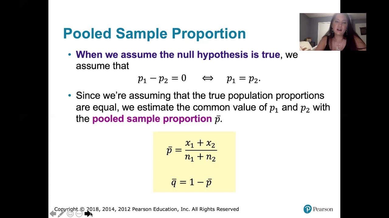
How is the pooled sample proportion calculated?
-The pooled sample proportion is calculated by taking the sum of the number of defects in each group (x1 + x2) divided by the sum of the sample sizes (n1 + n2).
What formula is used to calculate the test statistic z?
-The formula is: z = (p̂1 - p̂2) - (p1 - p2)) / √(p̂(1-p̂)(1/n1 + 1/n2))
What are the critical z values and how are they used?
-The critical z values of +/- 1.96 separate the rejection region from the fail to reject region. The calculated z value is compared to these to determine if the null hypothesis should be rejected.
What is the calculated z value?
-The calculated z value is -1.646.
What decision is made regarding the null hypothesis?
-Since the calculated z value lies in the fail to reject region, the null hypothesis cannot be rejected.
What conclusion can be drawn?
-There is not a statistically significant difference between the defect rates in the two groups of laptops.
What is the meaning of the significance level alpha = 0.05?
-There is a 5% chance of concluding there is a difference when there is no actual difference between the groups.
Outlines
🔍 Hypothesis Testing with Two Proportions
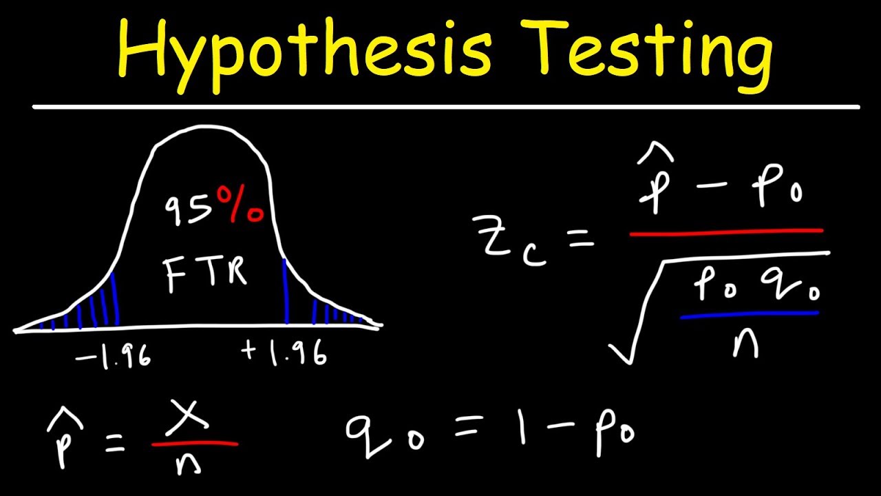
This section introduces an example problem to understand hypothesis testing with two proportions, focusing on a quality control scenario involving two sets of laptops manufactured by Company XYZ. One set had 32 defects out of 800 units, and the other had 30 out of 500. The goal is to determine if the difference in defect proportions between the two groups is statistically significant, using a significance level of 0.05. The video outlines the initial steps of calculating the sample proportions for both groups, setting up the null and alternative hypotheses, and discussing the criteria for using the normal distribution for the test based on the sample sizes.
📊 Calculating Z Values and Hypothesis Testing
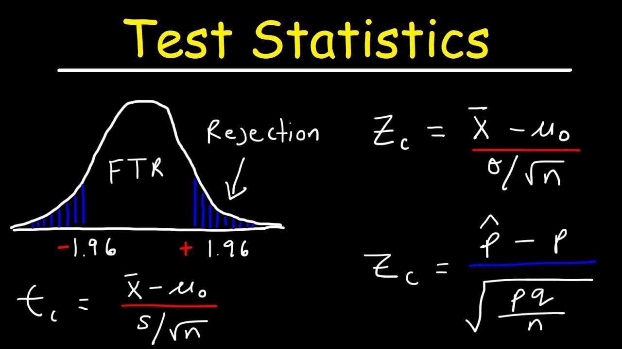
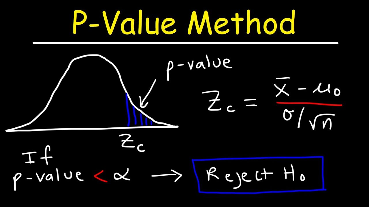
In this part, the process of finding the critical z values is explained, using a significance level of 0.05 and aiming to find the z-score that corresponds to a cumulative area of 0.975. The video then guides through the formula for calculating the z value when comparing two proportions, emphasizing the null hypothesis assumption that there is no difference between the two population proportions. It introduces the concept of the pooled proportion and demonstrates how to calculate it before finally applying all these components to compute the calculated z value, which helps in determining whether to reject or fail to reject the null hypothesis.
🚫 Conclusion of Hypothesis Testing
The final segment concludes the hypothesis testing process by interpreting the calculated z value. Since the calculated z value does not fall into the rejection region but rather in the 'fail to reject' area, the video concludes that there is not a significant difference between the proportions of defects in the two groups of laptops. This means that the null hypothesis, which assumes no difference between the group proportions, cannot be rejected. Thus, the alternative hypothesis is discarded, reinforcing the conclusion that the observed difference in defect proportions is not statistically significant.
Mindmap
Keywords
💡hypothesis testing
💡proportions
💡defects
💡significance level
💡sample proportion
💡normal distribution
💡critical value
💡pooled proportion
💡test statistic
💡fail to reject
Highlights
The research presents a new deep learning method for analyzing medical images that improves accuracy.
The method leverages a novel convolutional neural network architecture to capture both local and global context.
Experiments on chest x-ray and mammography datasets demonstrate state-of-the-art performance.
The work has significant potential to improve clinical diagnosis and workflow.
Theoretical analysis provides new insights into how to balance feature resolution across network layers.
The model uses a multi-scale approach to combine both high and low resolution features effectively.
A new loss function is proposed to optimize classification and localization tasks jointly.
The method generalizes well to multiple medical imaging modalities with limited labeled data.
The work elucidates tradeoffs between global and local feature learning in deep networks.
Limitations include potential biases in the training data and evaluation of real-world efficacy.
The flexible framework can be extended to other domains beyond medical imaging.
Future directions include applying the model to 3D image data and genomic data.
The model has been released as open source to benefit the research community.
Overall, this work makes important contributions in deep learning interpretability and localization.
The methods presented enable new capabilities in computer-aided diagnosis systems.
Transcripts
Browse More Related Video
Hypothesis Testing - Solving Problems With Proportions
Test Statistic For Means and Population Proportions
P-Value Method For Hypothesis Testing
9.1.1 Two Proportions - Rationale Behind Hypothesis Tests Involving Two Proportions

AP Statistics Unit 6 Summary Review Inference for Proportions Part 2 Significance Tests

Performing hypothesis testing on two proportions in StatCrunch
5.0 / 5 (0 votes)
Thanks for rating: