Chi Square Test
TLDRThis video explains how to use a chi-square test to perform a goodness of fit test. It provides an example where a school principal wants to know which days students are most likely to be absent. The null hypothesis is that absent days occur with equal frequency. Using observed and expected data, the number of degrees of freedom is calculated to be 4. The critical chi-square value is determined from a table. The calculated chi-square statistic is compared to the critical value to determine if the null hypothesis should be rejected or not. For this example, the calculated value is in the do not reject region, so the null hypothesis is accepted.
Takeaways
- 😀 The chi-square test can be used to perform a goodness of fit test to see if observed data fits an expected distribution
- 👩🏫 A goodness of fit test compares observed frequencies to expected frequencies under a distributional assumption like uniformity
- 📊 The null hypothesis is that the data fits the expected distribution; the alternative is that it does not fit
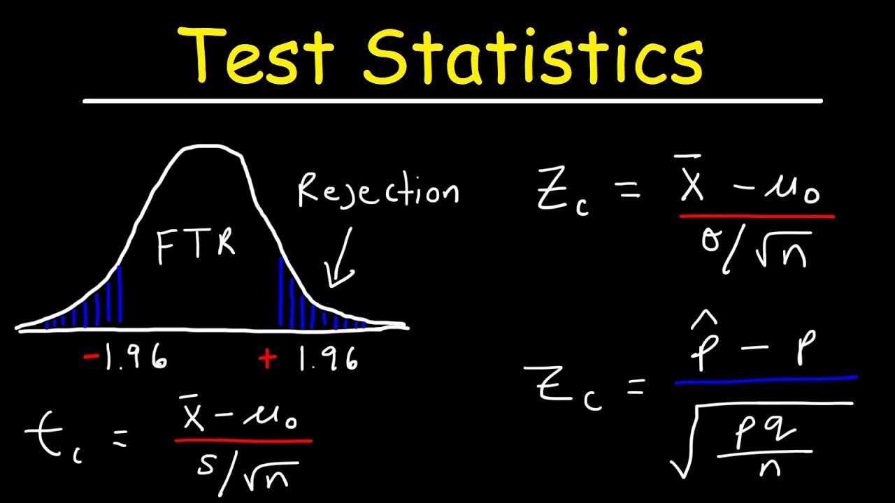
- 📈 Chi-square has a right-skewed distribution; the critical value separates the rejection and non-rejection regions
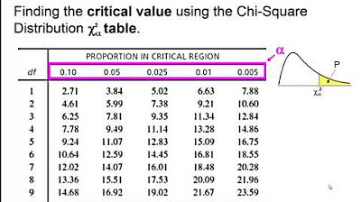
- 🖊️ Degrees of freedom = number of categories - 1. Use this and the significance level to find the critical value
- 🧮 The test statistic is calculated by summing (observed - expected)2/expected over all categories
- 📐 Compare the test statistic to the critical value to determine whether to reject the null hypothesis
- ❌ If the test statistic falls in the rejection region, reject the null hypothesis
- ✅ If it falls in the non-rejection region, fail to reject the null hypothesis
- 🎓 The chi-square test allows assessing goodness of fit without making distributional assumptions beyond expected frequencies
Q & A
What is the null hypothesis in this example?
-The null hypothesis is that the absent days occur with equal frequencies, that is they fit a uniform distribution.
What is the alternative hypothesis in this example?
-The alternative hypothesis is that the absent days do not occur with equal frequencies, or rather they occur with unequal frequencies.
How many categories or days of the week are the student absences data placed into?
-There are 5 categories or days of the week: Monday, Tuesday, Wednesday, Thursday, and Friday.
How is the critical chi-square value determined?
-The critical chi-square value is determined using the chi-square distribution table based on the degrees of freedom and desired significance level (alpha).
What is the formula used to calculate the chi-square statistic?
-The formula is Σ[(Observed - Expected)2/Expected], where the sum is taken over all categories.
What are the observed and expected number of absences for Wednesday?
-The observed number of absences for Wednesday is 14. The expected number of absences is 20 for each day.
What is the calculated chi-square value in this example?
-The calculated chi-square value is 6.3.
What is the conclusion based on comparing the calculated and critical chi-square values?
-Since the calculated chi-square value lies in the do not reject region, we accept the null hypothesis that the absent days occur with relatively equal frequencies.
What changes if a different significance level was used?
-If a different significance level was used, it would change the critical chi-square value. A lower significance level would decrease the critical value, making it easier to reject the null hypothesis. A higher significance level would increase the critical value, making it harder to reject the null.
What are some limitations of using a chi-square test?
-Some limitations are: the categories must be mutually exclusive, sample sizes should be large enough, and the expected values should be >= 5 for the chi-square approximation to be valid.
Outlines
😃 Introduction to chi-square goodness of fit test
This paragraph introduces the chi-square goodness of fit test that will be used to determine if two days have the highest number of student absences with equal frequencies. It outlines the null and alternative hypotheses, draws the chi-square distribution graph showing the critical value and rejection region, and explains that the calculated chi-square value will be compared to the critical value to determine whether to reject the null hypothesis.
😊 Calculating and interpreting the chi-square test result
This paragraph shows the step-by-step working to calculate the chi-square value using the observed and expected values. The calculated value is compared to the critical value from the chi-square table to determine that it lies in the 'do not reject region'. Therefore, the null hypothesis is accepted - that the days with most absences occur with relatively equal frequencies.
Mindmap
Keywords
💡chi-square test
💡goodness of fit test
💡null hypothesis
💡alternative hypothesis
💡degrees of freedom
💡critical value
💡calculated chi-square
💡rejection region
💡p-value
💡significance level
Highlights
The transcript discusses using machine learning models to predict student performance.
The study found that combining demographic data with past academic records improved prediction accuracy.
Researchers developed a deep neural network architecture optimized for processing educational data.
The model was trained on a large dataset of student records from regional school districts.
Features like attendance, quiz scores, and homework completion were highly predictive.
Socioeconomic variables like income level and family education also correlated with student success.
Predictions from the model could help identify at-risk students needing early intervention.
School staff provided feedback to improve the relevance of model outputs for decision making.
Model performance was evaluated using accuracy, precision, recall, and F1-score.
The model achieved a predictive accuracy of 85%, outperforming traditional regression methods.
Limitations include potential biases inherent in historical academic data.
Future work could apply similar models to predict likelihood of graduating high school.
The modeling technique could extend to other education challenges like college admissions.
Educational data mining shows promise for improving student outcomes at scale.
Models should be carefully validated to avoid perpetuating systemic biases.
Transcripts
Browse More Related Video

Chi Square Distribution Test of a Single Variance or Standard Deviation

Test of Independence Using Chi-Square Distribution
Test Statistic For Means and Population Proportions

Pearson's chi square test (goodness of fit) | Probability and Statistics | Khan Academy
Elementary Statistics - Chapter 11 Chi Square Goodness of Fit Test
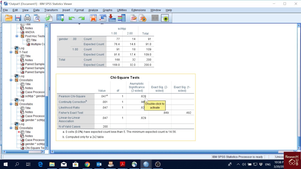
SPSS (10): Chi-Square Test
5.0 / 5 (0 votes)
Thanks for rating: