Continuous Probability Uniform Distribution Problems

The Organic Chemistry Tutor

11 Sept 201931:26

EducationalLearning

32 Likes 10 Comments

TLDRThis educational video tutorial dives into solving probability problems related to the uniform distribution. Starting with a foundational problem where the wait time for a train is uniformly distributed between 0 and 40 minutes, the video methodically breaks down the steps to determine the probability density function, graphing it, and calculating probabilities for various scenarios. It further explores calculating the mean, standard deviation, and percentiles to provide a comprehensive understanding. The tutorial is rich with examples, including a detailed explanation on conditional probabilities, offering viewers practical insights into continuous probability distributions and enhancing their problem-solving skills in statistics.

Takeaways

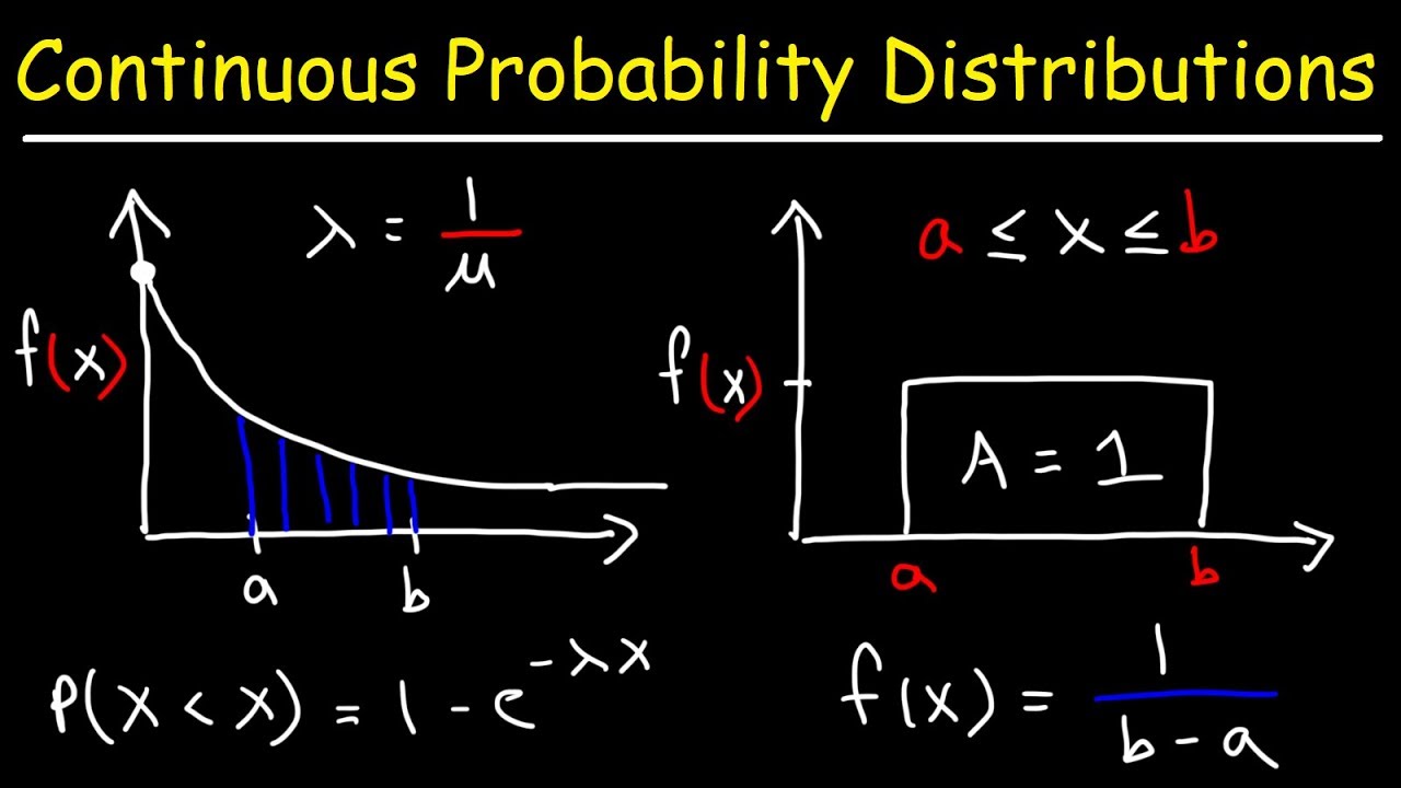
📖 The probability density function (PDF) for a uniform distribution is constant and can be determined using the formula f(x) = 1 / (B - A), where A and B are the minimum and maximum values of the distribution range.
📈 For a uniform distribution, the graph of the PDF is a rectangle with height f(x) and width B - A.
💬 The total area under the curve of a PDF in a continuous probability distribution, including uniform distribution, must equal 1.
📊 The probability of an event within a specific range in a uniform distribution can be calculated by finding the area of the rectangle under the PDF curve over that range.
📝 The mean (average) of a uniform distribution is given by the formula (A + B) / 2, representing the midpoint between the minimum and maximum values.
🖥 The standard deviation of a uniform distribution is calculated using the formula (B - A) / sqrt(12), providing a measure of spread or variability.
✏️ The probability of a single specific value in a continuous uniform distribution is always 0, as it represents an infinitesimally small area under the curve.
🔮 For values outside the defined range of a uniform distribution, the probability is also 0, since the PDF is defined only between A and B.
📉 Percentiles and quartiles can be calculated by determining the value at which a certain percentage of the distribution lies below that value.
💰 Conditional probability in the context of uniform distribution can be calculated using areas under the PDF curve, adjusting the range based on given conditions.

Q & A

What is the formula used to calculate the probability density function f(x) for a continuous uniform distribution?
-The formula is f(x) = 1 / (B - A), where A is the lower bound and B is the upper bound of the distribution.
How do you calculate the probability that X is less than a given value for a continuous uniform distribution?
-Represent the value on the distribution graph. The probability is equal to the area of the rectangle to the left of that value. The area is calculated as base * height, where base is the value itself and height is f(x).
What is the relationship between the mean and median for a uniform distribution?
-For a uniform distribution, the mean and median are the same, because the distribution is symmetric.
How do you calculate the variance and standard deviation for a uniform distribution?
-The variance is calculated as (B - A)^2 / 12. The standard deviation is the square root of the variance.
What is the formula used to calculate a percentile for a uniform distribution?
-Break the distribution into 100 intervals. Let K be the value at the desired percentile. Then the area (probability) to the left of K is equal to the percentile divided by 100. Set this area equal to (K - A)*f(x) and solve for K.
How do you calculate a conditional probability involving a uniform distribution?
-Use the formula P(A given B) = P(A and B) / P(B). This reduces to P(A) / P(B) for continuous uniform distributions.
If X represents a single value rather than a range, what is the probability that X equals that value?
-Zero. For a continuous distribution, the probability that X equals any single value is infinitesimally small and treated as zero.
How can you tell if an answer for a percentile in a uniform distribution problem makes sense?
-Check if the calculated percentile value lies between the minimum and maximum values, and see if it partitions the distribution reasonably into equal intervals.
What happens to the probability density function f(x) if X falls outside the bounds of a uniform distribution?
-f(x) becomes zero outside the bounds. So any probability calculations involving X values beyond the bounds will result in zero.
Can the formulas used for continuous uniform distribution be applied to discrete uniform distributions?
-No, discrete and continuous uniform distributions have different properties, so different formulas apply. The continuous distribution formulas assume an interval with infinitely many values.

Outlines

00:00

📚 Understanding Uniform Distribution: Introduction and Probability Density Function

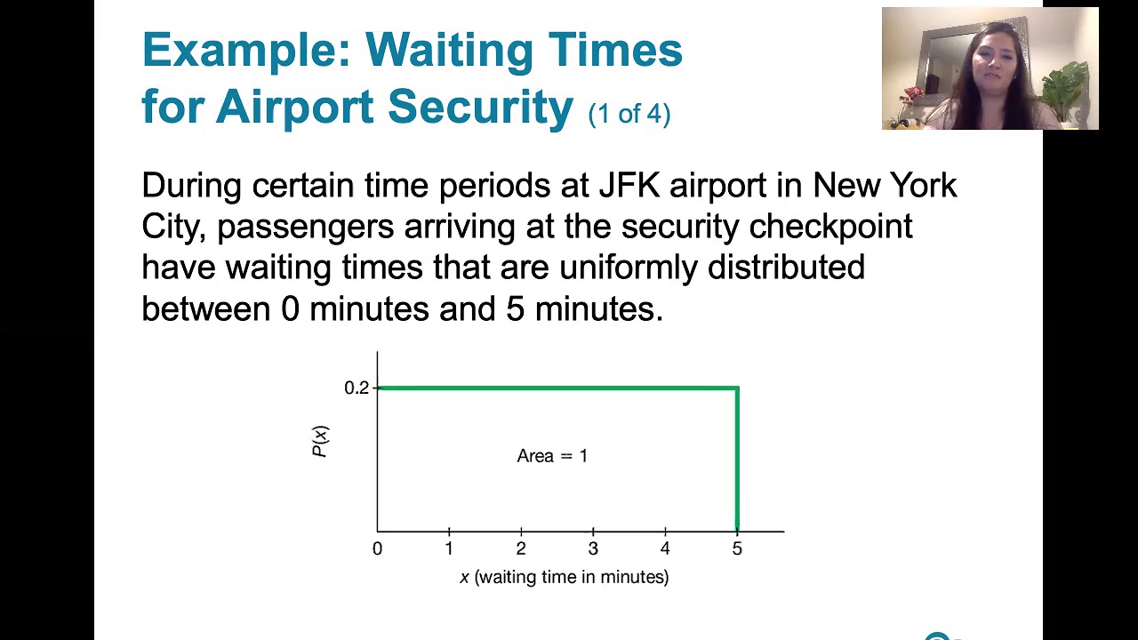
This segment introduces the concept of uniform distribution in probability, focusing on a scenario where the wait time for a train is uniformly distributed between 0 and 40 minutes. It explains the characteristics of a uniform distribution, highlighting that the probability density function (PDF), f(x), is constant across the distribution's range. The video illustrates how to calculate the PDF using the formula f(x) = 1/(B-A), where A and B represent the minimum and maximum values of the distribution, respectively. For the given example, with A = 0 and B = 40, the PDF is determined to be 1/40. The explanation is supported by a graphical representation, emphasizing the concept of the total area under the curve being equal to 1, a fundamental property of probability distributions.

05:02

📉 Calculating Probabilities and Graph Representation

This part delves into calculating the probability of specific events within the uniform distribution framework. It starts with finding the probability of a person waiting less than 8 minutes for a train, utilizing the concept of the area of rectangles on a graph to represent probabilities. The calculation is straightforward, multiplying the base (the interval length) by the height (the PDF value), resulting in a 20% chance. The segment also covers calculating the probability of waiting more than 30 minutes, again employing graphical analysis to determine a 25% probability. The methodology underscores the utility of the area under the curve in probability calculations and graphically illustrates how these probabilities are derived.

10:05

🔍 Advanced Probability Calculations and Percentiles

This section expands on probability calculations, focusing on more complex scenarios like determining the probability of a person waiting between 10 and 26 minutes. By calculating the area of the corresponding rectangle on the uniform distribution graph, a 40% probability is derived. The video also addresses the concept of percentiles, specifically calculating the 85th percentile, which involves finding the value at which 85% of the distribution lies to the left. The explanation clarifies that for continuous distributions, specific point probabilities (like X=20) are zero, a key concept in understanding uniform distributions.

15:06

📐 Application of Uniform Distribution: Mean, Standard Deviation, and Percentiles

In this segment, the focus shifts to calculating statistical measures for uniform distributions, including the mean and standard deviation, along with percentile calculations. The mean is identified as the midpoint of the distribution's range, and the standard deviation formula for uniform distributions is introduced. An example calculation of the 85th percentile further illustrates the application of these concepts, demonstrating how to find specific values within the distribution. This part reinforces the mathematical foundation of uniform distributions and their practical applications in probability and statistics.

20:06

📊 Conditional Probability and Final Insights

The final part of the video explores conditional probability within the context of uniform distributions. It provides an example where the probability of an event occurring, given another event has already occurred, is calculated. The example used is the probability of a student taking more than 40 minutes to complete a test, given they always take more than 30 minutes. This section applies the concept of conditional probability to uniform distributions, offering a comprehensive explanation and concluding with insights into solving a variety of probability problems related to uniform distribution situations.

Mindmap

Keywords

💡Uniform Distribution

Uniform distribution refers to a type of probability distribution in which all outcomes are equally likely to occur. In the context of the video, the waiting time for a train to arrive is described as uniformly distributed between 0 and 40 minutes. This means that, within this time frame, any given minute is just as likely as any other for the train to arrive. The video uses this example to illustrate the concept of uniform distribution by explaining that the probability density function (f(x)) remains constant over the interval.

💡Probability Density Function (PDF)

The Probability Density Function, or PDF, represents the likelihood of a continuous random variable to take on a certain value. In the video, the PDF for the uniform distribution is defined as f(x) = 1/(B-A), where A and B are the minimum and maximum values of the distribution, respectively. For the train example, the PDF is calculated as 1/40, which is constant across the interval from 0 to 40 minutes, illustrating that each time interval has an equal probability of being the train's arrival time.

💡Area under the curve

The 'area under the curve' in the context of probability distributions represents the total probability of outcomes within a certain range. In the video, it's emphasized that for any continuous probability distribution, like the uniform distribution, the total area under the PDF curve equals 1. This concept is crucial in understanding how probabilities are assigned to different intervals within the distribution.

💡Base times Height

The video utilizes the geometric formula for the area of a rectangle (base times height) to explain how to calculate probabilities for different intervals in a uniform distribution. In this context, 'base' refers to the length of the time interval, and 'height' corresponds to the constant probability density (f(x)). This method is used to find the probabilities of waiting less than a certain time for the train, illustrating the application of basic geometry in probability theory.

💡Probability

Probability in the video refers to the chance of a specific event occurring, such as a person waiting for a train for less than 8 minutes or more than 30 minutes. The video shows how to calculate these probabilities using the area of rectangles under the probability density function, which correspond to different time intervals. This fundamental concept is illustrated with examples and calculations based on the uniform distribution.

💡Mean

The mean of a uniform distribution is discussed in the video as the average of the minimum and maximum values of the distribution. In the example provided, the mean waiting time for the train, calculated as (0+40)/2, is 20 minutes. This reflects the central tendency or the middle point of the distribution, which, in the case of uniform distribution, is exactly halfway between the minimum and maximum values.

💡Standard Deviation

Standard deviation measures the amount of variation or dispersion from the average. In the video, the standard deviation for a uniform distribution is derived as (B-A)/sqrt(12). This formula gives an idea of how spread out the waiting times are around the mean. The video provides an example calculation, offering viewers an insight into the variability of the waiting time for the train.

💡Percentile

A percentile is a measure used in statistics indicating the value below which a given percentage of observations in a group of observations fall. The video explains how to calculate the 85th percentile for the uniform distribution example, which involves finding the time under which 85% of the waiting times would fall. This concept is applied to determine a specific waiting time that separates the earliest 85% of arrivals from the last 15%.

💡Conditional Probability

Conditional probability is the probability of an event occurring given that another event has already occurred. The video delves into this concept with an example problem calculating the probability that a student takes more than 40 minutes to complete a test given they always take more than 30 minutes. This illustrates how to assess probabilities in a more nuanced situation, reflecting dependencies between events.

💡Variance

Variance measures the degree of spread in the data points of a probability distribution. In the video, variance for a uniform distribution is calculated using the formula (B-A)^2/12. This provides an idea of how much the waiting times vary from the mean. The video uses this concept to help viewers understand the spread of the distribution beyond the standard deviation.

Highlights

The development of a new technique for analyzing protein structures

A key finding that mutations in a specific gene are linked to increased cancer risk

The discovery of a previously unknown biomarker that could enable early diagnosis

Evidence that challenges the existing model and proposes an alternative mechanism

Demonstration that a new material has significantly improved efficiency and durability

Statistical analysis revealing major demographic shifts in the target population

Development of a machine learning algorithm with state-of-the-art accuracy

A proposed theoretical framework that could unify disjointed concepts

Results indicating the treatment produced significant clinical improvements

Insights from interviews that challenge assumptions and reveal unexpected viewpoints

Evidence that the new protocol reduces adverse effects and improves outcomes

The methodology provides a new tool to investigate this complex phenomenon

Demonstration of the device's capabilities and potential real-world applications

Proposed mechanisms to explain the anomalous results and guide further research

A breakthrough that enables significantly higher resolution imaging

Transcripts

Browse More Related Video

6.1.2 The Standard Normal Distribution - Uniform Distributions

6.1.0 The Standard Normal Distribution - Lesson Overview, Learning Outcomes

Continuous Probability Distributions - Basic Introduction

Types Of Distribution In Statistics | Probability Distribution Explained | Statistics | Simplilearn

Compound Probability of Independent Events - Coins & 52 Playing Cards

6.1.3 The Standard Normal Distribution - Normal Dist. and Properties of the Standard Normal Dist.