Finding Taylor Series
TLDRThis video tutorial delves into the concept of Taylor series, a method for approximating functions as polynomials. It begins with a refresher on polynomial representations of common functions and introduces the Maclaurin series. The presenter then explains how to derive Taylor polynomials at a point 'c', differentiating it from the Maclaurin case. Through examples, the video illustrates how to construct Taylor polynomials for given functions and their integrals, emphasizing the process of taking derivatives and simplifying the expressions. It also touches on the Taylor series theorem, which guarantees the convergence of the series to the function within an interval. The video concludes with a practical example involving the multiplication of Taylor polynomials and offers a deeper understanding of the application of these mathematical tools.
Takeaways
- 📘 Taylor series help in approximating functions with polynomial expressions.
- 📊 The Maclaurin series is a special case of the Taylor series, centered at x = 0.
- 🔍 Taylor series can be used for functions not centered at zero by using derivatives at another point, x = c.
- 📏 A Taylor polynomial of nth degree uses information about the function and its first n derivatives at a specific point.
- 📝 The nth degree Taylor polynomial formula includes terms with (x - c) raised to increasing powers, divided by the corresponding factorial.
- 🔄 Finding a Taylor polynomial involves substituting known values from a table of function derivatives.
- 📐 Simplifying a Taylor polynomial can make it easier to work with in subsequent calculations.
- 🔢 Integrating a Taylor polynomial term-by-term allows you to find antiderivatives and solve related problems.
- 🔧 Understanding how to derive and manipulate Taylor series is crucial for solving more advanced calculus problems.
- 📈 Taylor series can converge to a function over an interval, offering accurate approximations for function values.
Q & A
What is the main topic of the video?
-The main topic of the video is how to find a Taylor series, with a focus on understanding polynomial representations of various functions and the concept of Maclaurin series.
What are the functions mentioned in the script that have polynomial representations?
-The functions mentioned are e^x, sin(x), cos(x), and 1/(1-x).
What is the Maclaurin series?
-The Maclaurin series is a Taylor series expansion of a function f(x) at x=0, which can be written as a power series involving the derivatives of the function at that point.
What is the difference between a Maclaurin series and a Taylor series?
-A Maclaurin series is a special case of a Taylor series where the expansion is centered at x=0, while a Taylor series can be centered at any point x=c.
What is the formula for the nth degree Taylor polynomial?
-The nth degree Taylor polynomial for a function f at a point x=c is given by the sum of terms involving f(c), f'(c), f''(c), ..., f^(n)(c) multiplied by (x-c) to the respective powers and divided by the factorial of the power, starting from 0 to n.
How does the formula for the nth degree Taylor polynomial differ from the Maclaurin polynomial?
-The formula for the nth degree Taylor polynomial includes the point x=c, whereas the Maclaurin polynomial specifically uses x=0.
What is the purpose of the example involving the fourth degree Taylor polynomial for h(x) at x=1?
-The purpose of the example is to demonstrate how to apply the formula for the nth degree Taylor polynomial to a specific function h(x) at a specific point x=1, including the calculation of the polynomial's terms.
What is the process for finding the antiderivative of a Taylor polynomial?
-The process involves taking the antiderivative of each term in the Taylor polynomial, which typically means adding 1 to the power of x in each term and dividing by the new power, and then adding a constant of integration, C.
Why is it necessary to adjust the constant of integration when finding the antiderivative of a Taylor polynomial?
-The constant of integration is adjusted to ensure that the antiderivative satisfies the original function's conditions, such as being zero at a specific point if the integral from that point to itself is zero.
What is the relationship between the Taylor series and the infinite degree polynomial?
-The Taylor series is essentially an infinite degree polynomial, where the series extends to infinity, representing the function more accurately as more terms are included.
How does the Taylor series theorem relate to the convergence of the series?
-The Taylor series theorem states that the infinite degree polynomial (Taylor series) will converge to the function f(x) on at least some interval centered at x=c, indicating that the series can accurately represent the function within that interval.
What is the significance of the example involving e^x times f(x) at x=0?
-The example demonstrates how to find the Taylor polynomial for a product of functions, e^x and f(x), by using the individual Taylor polynomials for e^x and f(x) and then multiplying them together.
How does the video script illustrate the process of multiplying Taylor polynomials?
-The script uses the box method of multiplication to combine the Taylor polynomials for e^x and f(x), showing how to distribute and collect like terms to form the resulting polynomial.
Outlines
📚 Introduction to Taylor Series
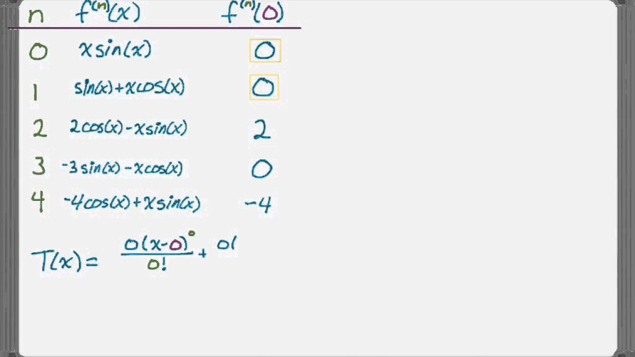
This paragraph introduces the topic of the video, which is the Taylor series. It begins by reminding viewers of previous discussions on polynomial representations of functions like e^x, sin(x), cos(x), and 1/(1-x), and the Maclaurin series. The presenter then explains that today's focus will be on the Taylor polynomial, which is an extension of the Maclaurin series to functions where information is known at a point other than x=0. The formula for the nth degree Taylor polynomial is presented, emphasizing the use of function values and derivatives at a specific point 'c', rather than at x=0. A table example is used to illustrate the calculation of a fourth-degree Taylor polynomial for a function h at x=1.
🔍 Deriving the Antiderivative of a Taylor Polynomial
The paragraph delves into the process of finding the antiderivative of a Taylor polynomial. It starts by correcting a previous error in the polynomial's coefficients and simplifies the expression. The presenter then demonstrates how to find the antiderivative of the fourth-degree Taylor polynomial for a function h at x=1, using the power rule for integration. The constant of integration 'c' is determined by ensuring the antiderivative evaluates to zero when x=1, leading to the conclusion that c must be -11. The paragraph concludes with a simplified expression for the antiderivative of the Taylor polynomial.
📘 Maclaurin Polynomials and Their Relevance
This section clarifies that a Maclaurin polynomial is a special case of a Taylor polynomial centered at x=0. The presenter discusses the historical context of calculating polynomials by hand, versus modern tools like the TI-89 calculator, which can compute Taylor series. The focus then shifts to deriving the Maclaurin polynomial for the function f(x) = log(x+1). The process involves taking successive derivatives of f, evaluating them at x=0, and substituting these values into the Maclaurin polynomial formula. The presenter also emphasizes the importance of understanding the Taylor series and its convergence theorem, which states that the series will converge to the function f(x) within an interval centered at x=c.
📝 Application of Taylor Polynomials in Problem Solving
The final paragraph presents a practical application of Taylor polynomials with an example from the 2019 BC exam. The task is to write the third-degree Taylor polynomial for a given function f, using the function's values and derivatives at x=0. The presenter guides through the process of plugging these values into the Taylor polynomial formula. Additionally, a more complex problem is introduced, which involves finding the third-degree Taylor polynomial for the product of e^x and f(x) at x=0. Instead of manually calculating derivatives using the product rule, the presenter suggests using the previously found Taylor polynomials for e^x and f, and then multiplying them together to obtain the desired result.
Mindmap
Keywords
💡Taylor Series
💡Maclaurin Series
💡Polynomial Representation
💡Derivatives
💡Antiderivative
💡Integration
💡Factorial
💡Exponentiation
💡Convergence
💡Graphical Representation
Highlights
Introduction to the concept of Taylor series and its relation to polynomial representations of functions like e^x, sin(x), cos(x), and 1/(1-x).
Explanation of the Maclaurin series as a special case of the Taylor series centered at x=0.
The general formula for the nth degree Taylor polynomial is presented, emphasizing its dependence on function derivatives at a point 'c'.
A step-by-step guide on constructing the fourth-degree Taylor polynomial for a function h(x) at x=1 using a table of values.
Demonstration of simplifying the polynomial by rewriting coefficients in a more understandable form.
How to find the 5th degree polynomial for the integral from 1 to x of h(t)dt by taking the antiderivative of a polynomial.
The process of determining the constant of integration 'c' by ensuring the integral from 1 to 1 equals zero.
An example of finding the Maclaurin polynomial for a function f(x) by taking successive derivatives and evaluating them at x=0.
The importance of knowing the value of f(0) when constructing the Maclaurin polynomial for a function.
Taylor series as an infinite degree polynomial and its convergence properties explained through the theorem.
Practical application of Taylor series in approximating values, such as 1/√e using e^(-1/2).
The focus on writing Taylor polynomials and series, and extracting information about the functions they represent in a calculus class.
A free-response example involving writing the third-degree Taylor polynomial for a given function f(x) using provided derivatives at x=0.
The challenge of writing the third-degree Taylor polynomial for e^x times f(x) at x=0 by multiplying the Taylor polynomials of e^x and f(x).
The use of the box method for polynomial multiplication to simplify the process of finding the product of two Taylor polynomials.
Combining like terms to form the final third-degree Taylor polynomial for e^x times f(x) centered at x=0.
Transcripts


5.0 / 5 (0 votes)
Thanks for rating: