AP Calculus BC Lesson 10.11 Part 3

Elizabeth Fein

20 Feb 202320:37

EducationalLearning

32 Likes 10 Comments

TLDRThis video tutorial delves into Taylor and Maclaurin polynomials, focusing on free response questions that require familiarity with the general formulas for Nth Degree Taylor and Maclaurin polynomials. The video assumes prior knowledge from previous lessons and guides viewers through solving complex problems involving derivatives and approximations of functions. It covers various degrees of polynomials and demonstrates how to apply these mathematical concepts to real-world problems, such as approximating function values and calculating areas under curves.

Takeaways

📚 The video covers Taylor and Maclaurin polynomials, focusing on free response questions and their general formulas.
👓 Familiarity with Nth Degree Taylor and Maclaurin polynomials is assumed, with a suggestion to watch previous videos for a refresher.
📈 The video presents a problem involving a function f with known derivatives, and asks for the third-degree Taylor polynomial about x=0.
🔢 The third-degree Taylor polynomial is derived using given derivative values at x=0, leading to a specific polynomial expression.
📊 A graph of function f is used to determine values of f(0) and f'(0), aiding in the construction of the Taylor polynomial.
🌟 The video demonstrates how to approximate function values using Taylor polynomials, as shown with an approximation for f(0.1).
📝 Another problem involves a function G, with its derivative given as a function of f, and a request to find the third-degree Taylor polynomial for G about x=0.
🧩 The construction of the Taylor polynomial for G involves using the chain rule to find higher derivatives of G.
📐 The video concludes with an example of using the Taylor polynomial for G to approximate its value at x=1.8, emphasizing the approximation nature of Taylor polynomials.
🔍 The process of solving these problems involves a combination of algebraic manipulation, understanding of derivatives, and the application of Taylor polynomials.
🎓 The video serves as an educational resource for understanding and applying Taylor and Maclaurin polynomials in mathematical problem-solving.

Q & A

What is the main topic of the video?
-The main topic of the video is Taylor and Maclaurin polynomials, specifically focusing on third-degree Taylor polynomials and their applications in solving free response questions.
What are the general formulas for Nth Degree Taylor and Maclaurin polynomials?
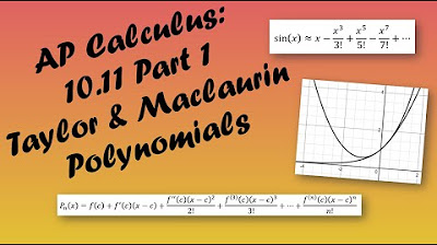
-The general formula for an Nth Degree Taylor polynomial is P_n(x) = f(a) + f'(a)(x-a) + f''(a)(x-a)^2/2! + ... + f^(n)(a)(x-a)^n/n!. For Maclaurin polynomials, which are Taylor polynomials centered at x=0, the formula simplifies to P_n(x) = f(0) + f'(0)x + f''(0)x^2/2! + ... + f^(n)(0)x^n/n!.
What is the significance of the third derivative of a function in the context of this video?
-The third derivative of a function is used in constructing the third-degree Taylor polynomial. It contributes to the term x^3/3! in the polynomial, which helps in approximating the function more accurately near the center point, in this case, x=0.
How does the video demonstrate the use of Taylor polynomials in solving free response questions?
-The video demonstrates the use of Taylor polynomials by walking through the process of finding the third-degree Taylor polynomial for a given function, using provided derivative information and a graph. It then applies this polynomial to approximate function values at specific points.
What is the role of the second derivative in the Taylor polynomial approximation?
-The second derivative plays a role in the second term of the Taylor polynomial, which is x^2/2!. It helps in the quadratic behavior of the polynomial, improving the approximation of the function near the center point.
How does the video address the concept of a horizontal tangent line?
-The video addresses the concept of a horizontal tangent line by discussing its implications for the second derivative of the function. A horizontal tangent line at x=0 means that the second derivative, and consequently the coefficient of the x^2 term in the Taylor polynomial, is zero.
What is the significance of the area under the curve in the context of the integral provided in the video?
-The area under the curve, given as 1.518, is used to find the value of G(0) in the Taylor polynomial for the function G(x). Since G(x) is defined as an integral of f(t) from 2 to x, the area under the curve from 0 to 2 represents the value of G(0).
How does the video use the differential equation to find the first derivative of the function?
-The video uses the given differential equation dy/dx = y * ln(x) with the initial condition f(1) = 4 to find the first derivative at x=1. By substituting x=1 and y=4 into the equation, the video determines that f'(1) = 0, as the natural log of 1 is zero.
What is the purpose of the second-degree Taylor polynomial for G(x) in the video?
-The second-degree Taylor polynomial for G(x) is used to approximate the value of G(1.8). By plugging in x=1.8 into the polynomial, the video provides an approximation of the function value at that point.
How does the video ensure clarity in the explanation of Taylor polynomials?
-The video ensures clarity by breaking down the process of constructing Taylor polynomials step by step, explaining each term's contribution, and providing visual references to a graph. It also emphasizes the importance of notation and the inclusion of all terms, even those with zero coefficients.
What is the final approximation given for the function value at x=0.1 in the video?
-The final approximation given for the function value at x=0.1 is 9.515, obtained by evaluating the fourth-degree Taylor polynomial at x=0.1.

Outlines

00:00

📚 Introduction to Taylor and Maclaurin Polynomials

This paragraph introduces the topic of Taylor and Maclaurin polynomials, emphasizing the importance of understanding the general formulas for these polynomials. It mentions that the video will cover free response questions related to these topics and suggests that viewers familiarize themselves with the basics by watching previous videos if necessary. The paragraph sets the stage for a detailed exploration of Taylor and Maclaurin polynomials, highlighting the significance of these mathematical tools in approximating functions.

05:00

🔢 Solving Third Degree Taylor Polynomial Problems

The paragraph delves into the process of solving problems involving third degree Taylor polynomials. It explains the need to identify the degree of the polynomial and the center, which in this case is x equals zero, indicating a Maclaurin polynomial. The speaker provides a step-by-step guide on how to write the general formula for a third degree Taylor polynomial, how to determine the values of the function at the center, and how to plug these values into the formula. The paragraph also includes an example of finding the third degree Taylor polynomial for a given function and its derivatives.

10:02

📈 Approximating Function Values with Taylor Polynomials

This section focuses on using Taylor polynomials to approximate function values. It begins by outlining the general formula for a fourth degree Taylor polynomial centered at x equals zero and proceeds to plug in values for the derivatives to find the polynomial. The speaker then uses this polynomial to approximate the value of the function at x equals 0.1, demonstrating the practical application of Taylor polynomials in function approximation. The paragraph also touches on the process of simplifying the polynomial for easier computation.

15:05

🧮 Derivatives and Taylor Polynomials for Function G

The paragraph discusses the application of Taylor polynomials to a different function, G, which is related to function F through a derivative relationship. It explains how to find the third degree Taylor polynomial for G and how to use this polynomial to find the value of G at a specific point. The speaker provides a clear explanation of how to derive the formulas for the higher derivatives of G and how to plug these into the Taylor polynomial formula. The paragraph also includes the process of solving a differential equation to find one of the derivatives needed for the Taylor polynomial.

20:05

📊 Approximating Areas Under a Curve

This final paragraph discusses the application of Taylor polynomials in approximating areas under a curve. It introduces a function G defined as an integral of F, and explains how to find the second degree Taylor polynomial for G about x equals zero. The speaker then uses this polynomial to approximate the value of G at x equals 1.8. The paragraph also touches on the concept of the area between the curve and the x-axis, and how the Taylor polynomial can be used to approximate this area. The speaker emphasizes the approximation nature of Taylor polynomials, reminding viewers that they provide close estimates but not exact values.

Mindmap

Keywords

💡Taylor Polynomials

Taylor Polynomials are mathematical expressions used to approximate functions. They are constructed by taking the function's derivatives at a certain point, known as the center, and are particularly useful for functions that are differentiable. In the video, Taylor Polynomials are used to approximate the behavior of a function f around x=0 and x=1, with examples provided for third-degree and second-degree polynomials.

💡Maclaurin Polynomials

Maclaurin Polynomials are a special case of Taylor Polynomials where the center of expansion is at x=0. They are named after the Scottish mathematician Colin Maclaurin. These polynomials are used to provide approximations of functions that are at least twice differentiable at the center point. In the video, Maclaurin Polynomials are used to approximate the function f and another function G around x=0.

💡Derivatives

Derivatives represent the rate of change of a function with respect to its variable. They are fundamental to calculus and are used to analyze the behavior of functions, such as determining rates of change, maximums, and minimums. In the context of the video, derivatives are crucial for constructing Taylor and Maclaurin Polynomials, as these polynomials are built using the function's derivatives at a specific point.

💡Center

In the context of Taylor and Maclaurin Polynomials, the center refers to the point around which the polynomial is expanded. The choice of center affects the coefficients of the polynomial and thus its accuracy as an approximation. The video emphasizes the importance of identifying the center when working with these polynomials and uses x=0 as the center for constructing Maclaurin Polynomials.

💡Free Response Questions

Free response questions are open-ended problems that require students to provide a full answer, often with explanations or calculations. In the context of the video, these questions pertain to applying knowledge of Taylor and Maclaurin Polynomials to solve problems involving function approximation and finding derivatives.

💡Approximation

In mathematics, approximation involves finding a simpler function or value that is close to a more complex one. Taylor and Maclaurin Polynomials are tools used to approximate functions, particularly when an exact solution is not feasible or practical. The video demonstrates how these polynomials can be used to approximate the values of functions at specific points.

💡Graph

A graph is a visual representation of the relationship between variables, typically used in mathematics to illustrate the behavior of functions. In the context of the video, the graph of a function is used to visually identify certain properties of the function, such as its value at a point, the slope of the tangent line at a point, and the area under the curve.

💡Integral

An integral is a fundamental concept in calculus that represents the accumulation of a quantity, often understood as the area under a curve or the sum of an infinite series of values. Integrals are used to find the antiderivative of a function, which can help in solving differential equations and determining areas or volumes.

💡Differential Equation

A differential equation is an equation that relates a function and its derivatives. These equations are essential in modeling various phenomena in physics, engineering, and other fields. The video presents a first-order differential equation to find the derivative of a function f, which is then used to construct a Taylor Polynomial.

💡Tangent Line

A tangent line is a line that touches a curve at a single point and has the same slope as the curve at that point. Tangent lines are used in calculus to study the local behavior of functions, such as determining the rate of change or the instantaneous velocity at a given moment. In the video, the slope of the tangent line to a function at a specific point is used to find the first derivative of the function.

Highlights

Introduction to Taylor and Maclaurin polynomials as key concepts in calculus.

Explanation of the general formulas for Nth Degree Taylor and Maclaurin polynomials.

Discussion on the importance of understanding Taylor polynomials for free response questions.

Illustration of how to derive a third-degree Taylor polynomial for a given function.

Use of graph analysis to determine the value of f(0) and the derivatives at x=0.

Step-by-step calculation of the third-degree Taylor polynomial using provided derivatives.

Demonstration of solving for f(0) using first-degree Taylor polynomial and given P_sub_1 of 1/5.

Procedure for finding the fourth-degree Taylor polynomial and approximating f(0.1) using it.

Explanation of the relationship between a function G and its derivative G', as G'(x) = f(3x).

Method for calculating Q_sub_3 of x using the derivatives of G and the initial condition g(0).

Construction of a second-degree Taylor polynomial for a function f centered at x=1.

Use of differential equations to find the value of f'(1) and subsequently the Taylor polynomial.

Approximation of f(2) using the second-degree Taylor polynomial around x=1.

Definition of function G as the integral from 2 to x of f(t) dt and its relation to the area under the curve.

Derivation of G(0) using the integral and the area under the curve from 0 to 2.

Explanation of how to find G'(x) and its implications for the second-degree Taylor polynomial of G.

Application of the second-degree Taylor polynomial for G to approximate G(1.8).

Transcripts

Browse More Related Video

AP Calculus BC Lesson 10.11 Part 1

Finding Taylor Series

Avon High School - AP Calculus BC - Topic 10.11 - Example 2

AP Calculus BC Lesson 10.11 Part 2

Taylor Polynomials Day 1

Taylor Polynomials

Related Tags

Mathematics Calculus Taylor Polynomials Maclaurin Polynomials Derivatives Integrals Free Response Educational Content Problem Solving Math Tutorial