Avon High School - AP Calculus BC - Topic 10.11 - Example 2
TLDRThis educational video delves into the exploration of Taylor and Maclaurin polynomials, extending the idea of approximating functions with higher degree polynomials. The instructor starts by revisiting linear and quadratic models, then progresses to constructing a third degree polynomial, explaining the importance of matching derivatives for a reliable model. Through a detailed example with the natural log function, the concept of Taylor polynomials is introduced, attributed to Brook Taylor, alongside Maclaurin polynomials, which are centered at zero. The video culminates in applying these concepts to approximate the sine function, demonstrating the process with a seventh degree Maclaurin polynomial for sine of x, and showcasing the remarkable accuracy of this approximation method.
Takeaways
- 📚 The video is an instructional piece aimed at Calculus BC students, focusing on extending linear and quadratic models to higher degree polynomials.
- 📈 Introduces the concept of Taylor and Maclaurin polynomials, highlighting their use in approximating functions with polynomials of higher degrees.
- 🤖 Discusses the logical progression from linear (P1) and quadratic (P2) models to a third degree polynomial (P3), emphasizing the need to match function derivatives to ensure accuracy.
- 🖥 Explores the process of determining the coefficients of higher degree polynomials through derivatives, illustrating with the example of finding the constant 'b'.
- 📝 Defines Taylor polynomials and distinguishes them from Maclaurin polynomials by their centering point, with Maclaurin polynomials specifically centered at zero.
- ✏️ Provides a brief historical background on Brook Taylor and Colin Maclaurin, crediting them for the development of these polynomial approximations.
- 🚡 Demonstrates the application of Maclaurin polynomials through an example involving the sine function, explaining the step-by-step derivation up to the seventh degree polynomial.
- ⏳ Emphasizes the iterative nature of finding derivatives up to the desired degree, showing the cycle of sine and cosine derivatives to find the seventh degree polynomial.
- 📄 Highlights the importance of evaluating derivatives at zero for Maclaurin polynomials, simplifying the process of determining coefficients.
- 🚀 Showcases the accuracy of polynomial approximations by comparing the seventh degree polynomial's approximation of sine (0.2) to the actual sine value, noting an impressive degree of precision.
Q & A
What are Taylor and Maclaurin polynomials, and how are they related?
-Taylor and Maclaurin polynomials are methods used to approximate actual functions with polynomials. They are named after the English mathematicians Brook Taylor and Colin Maclaurin. A Taylor polynomial is centered at some value 'c', while a Maclaurin polynomial is specifically centered at zero. Both follow the pattern of using the nth derivative of a function over the nth factorial, multiplied by (x - c) to the n.
How do you determine the coefficients for a third-degree Taylor polynomial?
-The coefficients of a third-degree Taylor polynomial are determined based on satisfying the condition that the polynomial's derivatives up to the third order match those of the original function at a specific point. The coefficient 'b' for the cubic term is found by equating the third derivative of the polynomial to the third derivative of the function, solved by dividing the third derivative evaluated at 'c' by three factorial.
What is the significance of the factorial in the coefficients of Taylor polynomials?
-The factorial in the coefficients of Taylor polynomials plays a critical role in ensuring that the derivatives of the polynomial match the derivatives of the function at a specific point. It serves as a scaling factor that properly adjusts the influence of each term in the polynomial, allowing for an accurate approximation of the function.
Why are only odd-degree terms used in the Maclaurin polynomial for the sine function?
-In the Maclaurin polynomial for the sine function, only odd-degree terms are used because the derivatives of sine alternate between sine and cosine (and their negatives), which results in the even-degree derivatives being zero when evaluated at zero. This pattern leads to only the odd-degree terms having non-zero coefficients, thus contributing to the polynomial.
How does the Maclaurin polynomial approximation of sine(x) compare with the actual sine function?
-The Maclaurin polynomial approximation of sine(x) closely matches the actual sine function within a certain interval around the center of approximation, which is zero. The approximation's accuracy improves with the inclusion of higher-degree terms. For example, a seventh-degree polynomial can provide an approximation accurate to several decimal places for small values of x.
What does the process of finding a Maclaurin polynomial for a function involve?
-Finding a Maclaurin polynomial for a function involves calculating the function's derivatives up to the desired degree, evaluating these derivatives at zero, and then constructing the polynomial using these values as coefficients. Each term of the polynomial is of the form (nth derivative evaluated at 0)/(n factorial) times (x^n).
Why was a seventh-degree polynomial chosen for approximating sine(x) in the example?
-A seventh-degree polynomial was chosen for approximating sine(x) to demonstrate the process of polynomial approximation with a function that has a repeating derivative pattern. This high degree allows for a closer approximation and showcases the effectiveness of Taylor and Maclaurin polynomials in approximating trigonometric functions over an interval.
What distinguishes a Taylor polynomial centered at zero from a Maclaurin polynomial?
-While a Taylor polynomial can be centered at any value 'c', a Maclaurin polynomial is specifically a Taylor polynomial centered at zero. Essentially, a Maclaurin polynomial is a special case of the Taylor polynomial, with the distinction lying in the choice of the center point.
How accurate was the seventh-degree Maclaurin polynomial approximation of sine(0.2)?
-The seventh-degree Maclaurin polynomial approximation of sine(0.2) was highly accurate, matching the actual sine function value to several decimal places. This demonstrates the effectiveness of using higher-degree polynomials for function approximation near the point of expansion.
What pattern is observed in the terms of the seventh-degree Maclaurin polynomial for sine(x)?
-In the seventh-degree Maclaurin polynomial for sine(x), a pattern of odd-degree terms being present is observed. This reflects the nature of the sine function's derivatives, where only odd-degree terms contribute to the polynomial due to the alternating sine and cosine derivatives evaluated at zero.
Outlines
📚 Introduction to Higher Degree Polynomials and Taylor Polynomials
This paragraph delves into the concept of approximating actual functions using higher degree polynomials, building upon the introduction of linear and quadratic models from previous lessons. The focus is on extending the idea to include third, fourth, and higher power polynomials. The video emphasizes the importance of matching derivatives to ensure a reliable model. It introduces the construction of third-degree polynomials and the process of finding the value of the constant term 'b' by equating the third derivative of the polynomial to the third derivative of the function at a specific point 'c'. The paragraph concludes with the definition of Taylor and Maclaurin polynomials, highlighting their significance in mathematical approximations.
🔢 Derivation of Maclaurin Polynomials and their Application
The second paragraph explains the process of deriving Maclaurin polynomials, which are a special case of Taylor polynomials centered at zero. It outlines the steps to find the seventh-degree Maclaurin polynomial for the sine function, emphasizing the pattern of derivatives and their evaluation at zero. The paragraph details the calculation of each term in the polynomial and the resulting expression. It also discusses the difference between Taylor and Maclaurin polynomials, noting that while Taylor polynomials can be centered at any value 'c', Maclaurin polynomials are specifically centered at zero. The historical contributions of mathematicians Brook Taylor and Colin Maclaurin are acknowledged, providing context for the naming of these polynomials.
📈 Approximating Sine with a Seventh Degree Maclaurin Polynomial
This section demonstrates the practical application of the seventh-degree Maclaurin polynomial by using it to approximate the value of sine for x=0.2. The video walks through the process of evaluating the polynomial at this point and compares the result with the actual value of sine(0.2), highlighting the high degree of accuracy obtained. The paragraph also encourages viewers to pause and catch up if they fall behind, emphasizing the importance of understanding the process. The discussion extends to the observation of the degree of each term in the polynomial, noting that they are all odd powers, and prompts viewers to make a conjecture about the Maclaurin polynomial for the cosine function.
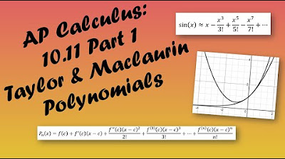
📊 Graphing the Seventh Degree Polynomial and Sine Function
The final paragraph of the script focuses on the visual representation of the seventh-degree polynomial and the sine function. It describes the process of graphing the polynomial and the sine function on a calculator, emphasizing the close match between the two, particularly around the x-value of 0.2. The video adjusts the graph to better illustrate the approximation quality, showing that the polynomial closely follows the sine curve. The paragraph concludes with a reflection on the historical significance of these mathematical tools and a teaser for future lessons, encouraging viewers to subscribe and continue learning about Taylor polynomials and their applications.
Mindmap
Keywords
💡Taylor Polynomials
💡Maclaurin Polynomials
💡Derivatives
💡Function Approximation
💡Factorial
💡Series Expansion
💡Convergence
💡Polynomial Degree
💡Function's Derivative Matching
💡Approximation Accuracy
Highlights
Introduction to higher degree polynomial models in calculus.
Explanation of linear and quadratic models mimicking the natural log function.
Discussion on extending models to third, fourth, and fifth power polynomials.
Derivation of a third-degree polynomial model and its conditions.
Explanation of matching the function and its derivatives with the polynomial model.
Clarification on the established conditions for second-degree polynomial usage.
Process of taking the third derivative to find the polynomial coefficient.
Introduction to Taylor and Maclaurin polynomials with historical context.
Definition of nth degree Taylor polynomials and their formulation.
Explanation of the specific case of Maclaurin polynomials centered at zero.
Application of seventh degree Maclaurin polynomial for sine function.
Derivative calculation for sine function to obtain polynomial coefficients.
Pattern recognition in polynomial term degrees and their significance.
Approximation of sine values using Maclaurin polynomial and its accuracy.
Graphical comparison of sine function and its seventh-degree polynomial approximation.
Transcripts


5.0 / 5 (0 votes)
Thanks for rating: