Mixed Design ANOVA
TLDRThis screencast offers a comprehensive guide on conducting and interpreting a mixed design ANOVA, focusing on a study that compares the body fat percentage changes over time in four groups of overweight individuals with different interventions. It covers the analysis process in SPSS, including assumptions, interaction effects, and post-hoc tests, and concludes with how to report the findings effectively.
Takeaways
- 📚 The screencast teaches how to conduct and interpret a mixed design ANOVA, which includes a within-subjects factor and a between-subjects factor.
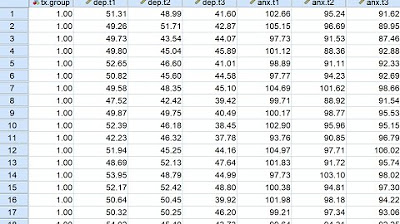
- 🔍 The example data involves the body fat percentage of four groups of overweight individuals measured at three time points: baseline, 6 months, and 12 months post-intervention.
- 📈 The mixed design ANOVA is used to evaluate changes in body fat percentage over time and to see if these changes differ between the four intervention groups.
- 📝 The assumptions of a mixed design ANOVA are similar to those of a repeated measures and one-way ANOVA, including sphericity and equality of error variances.
- 🛠️ The analysis is performed in SPSS using the General Linear Model, Repeated Measures, and defining the within-subject factor as 'time' with three levels.
- 📊 Profile plots are created in SPSS to visualize the interaction between time and group, which is crucial for interpreting the results.
- ✅ The results show significant changes over time in body fat percentage across the sample, indicating the effectiveness of the interventions.
- 🔑 A significant interaction between group and time suggests that the rate of body fat percentage reduction is not the same for all groups.
- 📉 Post-hoc tests, such as Tukey's HSD, are used to determine which specific groups differ significantly in their body fat percentage changes.
- 📋 Reporting results of a mixed design ANOVA includes presenting F values, degrees of freedom, and probability values for each effect and interaction.
- 📈 The final plot in the output helps interpret the interaction effect, showing how different groups' body fat percentage changes over time.
Q & A
What is the main focus of the screencast?
-The screencast focuses on teaching how to carry out and interpret a mixed design ANOVA (Analysis of Variance) test, including how to report the results of such a test.
What is the purpose of the experiment described in the script?
-The experiment aims to evaluate whether participants in different groups reduced their body fat percentage over time and if the reduction was more significant in some groups than others.
What are the four groups in the experiment?
-The four groups are control (no intervention), diet only, exercise only, and diet and exercise.
How many times were the participants' body fat percentages measured?
-The participants' body fat percentages were measured at three different occasions: at baseline, at the end of the 6-month intervention, and at the 12-month follow-up period.
What does the term 'mixed design ANOVA' refer to in the context of the script?
-In the script, 'mixed design ANOVA' refers to a statistical test that includes both a within-subject factor (time) with three levels and a between-subject factor (group) with four levels.
What assumptions should be checked for a mixed design ANOVA?
-The assumptions for a mixed design ANOVA include sphericity, homogeneity of variances, and normality of the data, similar to those for a repeated measures ANOVA and a one-way ANOVA.
How is the interaction between time and group represented in the script?
-The interaction between time and group is represented by the significant F value in the 'Time by Group' section of the ANOVA output, indicating that the changes in body fat percentage over time are not equivalent across the four groups.
What does the Mauchly's test of sphericity assess?
-The Mauchly's test of sphericity assesses the assumption of sphericity, which is the assumption that the variances of the differences between all possible pairs of within-subject conditions are equal.
What is the purpose of the profile plot in the context of the mixed design ANOVA?
-The profile plot is used to aid the interpretation of the interaction between time and group, showing how the mean scores of each group change over time.
How are post-hoc tests used in the script to analyze the significant interaction?
-Post-hoc tests, specifically Tukey's HSD (Honestly Significant Difference) test, are used to perform multiple comparisons for observed means to determine which specific group differences are statistically significant.
What is the significance of the reported p-values in the ANOVA output?
-The p-values indicate the probability that the observed effects (e.g., differences between group means or changes over time) occurred by chance. A p-value less than .05 typically indicates statistical significance.
How should the results of a mixed design ANOVA be reported in a text?
-The results should be reported by presenting the F value, its degrees of freedom, and the probability value for each significant effect (time, group, and their interaction). If the interaction is significant, the main effects should not be interpreted further, and the interaction plot should be described.
Outlines
📊 Mixed Design ANOVA Overview
This paragraph introduces the concept of a mixed design ANOVA (Analysis of Variance), also known as a repeated measures ANOVA with a between-subjects factor. The focus is on a study involving four groups of overweight individuals whose body fat percentage was measured at three time points: baseline, 6 months post-intervention, and at a 12-month follow-up. The aim is to determine if there's a reduction in body fat percentage over time and if this reduction varies across the groups, which include control, diet only, exercise only, and diet with exercise. The paragraph also explains the process of setting up such an analysis in SPSS, including defining within-subject factors (time) and between-subject factors (group), and how to create profile plots for interaction interpretation.
📈 Setting Up and Running the Analysis in SPSS
The second paragraph delves into the specifics of setting up a mixed design ANOVA in SPSS. It details the steps for defining factors, selecting the appropriate post-hoc tests for multiple comparisons, and adjusting for confidence intervals using the Bonferroni method. The paragraph also emphasizes the importance of checking for sphericity and equality of error variances to ensure the assumptions of the ANOVA are met. Descriptive statistics and the results of the Mauchly's test for sphericity are discussed, along with the interpretation of the test results, including the significance of the F values and P values in determining whether the variances are equivalent across groups and time points.
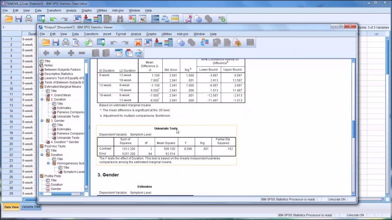
📉 Interpreting ANOVA Results and Post-Hoc Tests
This paragraph focuses on interpreting the results of the mixed design ANOVA. It explains the significance of the main effects for time and group, as well as the interaction effect between time and group. The paragraph guides through the process of examining the estimated marginal means and conducting pairwise comparisons to determine which time points differ significantly. It also discusses the interpretation of post-hoc tests, specifically the Tukey HSD test, to understand the differences between the groups and the control group, and how to report these findings accurately.
📊 Analyzing Changes Over Time and Group Differences
The fourth paragraph continues the analysis by examining the changes in body fat percentage over time and the differences between the groups. It discusses the significance of the interaction effect and the need to focus on this when interpreting the results. The paragraph also addresses how to modify the SPSS syntax for further analysis of the interaction effect and how to interpret the plot of the interaction. It emphasizes the importance of conducting follow-up tests to understand the specific differences between the groups at each time point.
📝 Reporting Results of Mixed Design ANOVA
The final paragraph concludes the screencast by outlining how to report the results of a mixed design ANOVA. It provides guidance on presenting the F values, degrees of freedom, and probability values for each effect and interaction. The paragraph also advises on the presentation of results in written format, figures, or tables, and stresses the importance of focusing on the significant effects and their implications. It concludes with a summary of the main findings from the study, highlighting the changes in body fat percentage over time and the differences between the groups.
Mindmap
Keywords
💡Mixed Design ANOVA
💡Within-Subjects Factor
💡Between-Subjects Factor
💡Interaction
💡SPSS
💡Assumptions
💡Descriptive Statistics
💡Post Hoc Tests
💡Estimated Marginal Means
💡Pairwise Comparisons
💡Effect Size
💡Homogeneity of Variance
Highlights
The screencast covers mixed design ANOVA, also known as repeated measures with a between-subject factor.
Participants' body fat percentage scores are analyzed across four groups and three time points.
The study aims to evaluate the reduction in body fat percentage over time and the interaction between group and time.
SPSS is used to carry out the mixed design ANOVA test with step-by-step instructions provided.
Assumptions of mixed design ANOVA are discussed, including sphericity and equality of error variances.
Descriptive statistics and significance tests for sphericity are presented in the SPSS output.
The test of within-subjects effects reveals significant changes over time in body fat percentage.
A significant interaction between group and time is found, indicating different rates of body fat reduction.
The main effect of group shows significant differences in body fat percentage across the four groups.
Post-hoc tests using Tukey's method are conducted to determine which groups differ significantly.
Estimated marginal means and pairwise comparisons are used to interpret changes over time within each group.
The control group shows no change in body fat percentage, while the other groups show a decrease.
The diet and exercise group had significantly lower body fat percentage compared to the diet-only and control groups.
Profile plots are used to visualize the interaction between time and group effects.
The screencast explains how to modify the SPSS syntax for further analysis of the interaction effect.
Guidance on reporting the results of a mixed design ANOVA, including F values, degrees of freedom, and probability values.
Instructions on how to present results in written, figure, or table format for clarity and understanding.
Transcripts
Browse More Related Video
How to Run One Way ANOVA in SPSS: Concept, Interpretation, and Reporting One Way ANOVA
Conducting a Two-Way ANOVA in SPSS

Duncan Multiple Range Test (DMRT) with Compact Letter Display

How to do a One-Way ANOVA in SPSS (12-6)

Pretest and Posttest Analysis with ANCOVA and Repeated Measures ANOVA using SPSS
Two-way repeated measures ANOVA in SPSS: one-within, one-between (March 2020)
5.0 / 5 (0 votes)
Thanks for rating: