AP Calculus AB: Lesson 2.6 Tangent Line Approximations

Michelle Krummel

11 Oct 202040:29

EducationalLearning

32 Likes 10 Comments

TLDRThis lesson delves into the concept of local linearization, illustrating how tangent lines can be utilized to approximate function values. The function g(x) = -x^2 + 3x + 2 serves as a basis to derive its tangent line and explore its slope at specific points. The instructor meticulously demonstrates the calculation of the derivative, the tangent line equation at x=2, and how to use the local linearization to estimate function values near a point of tangency. The video also explains the relationship between the function, its tangent line, and the implications of concavity on approximation accuracy, providing insights into when the tangent line may overestimate or underestimate function values.

Takeaways

📚 The lesson focuses on local linearization, which uses tangent lines to approximate function values.
🔍 The function \( g(x) = -x^2 + 3x + 2 \) is used to demonstrate the process of finding the derivative using the limit definition.
🧭 The derivative \( g'(x) \) is found to be \( -2x + 3 \) by simplifying the limit expression and factoring out \( h \).
📈 The slope of the tangent line at \( x = 2 \) is calculated to be \( -1 \) by substituting \( x = 2 \) into \( g'(x) \).
📝 The value of \( g(2) \) is determined to be 4 by substituting \( x = 2 \) into the original function \( g(x) \).
📉 The equation of the tangent line at the point (2, g(2)) is derived using the point-slope form, resulting in \( y - 4 = -1(x - 2) \).
📝 The concept of local linearization is introduced as an approximation method for differentiable functions near a point of tangency.
🔑 The local linearization is represented by the tangent line equation \( y = f(a) + f'(a)(x - a) \), which is an approximation of \( f(x) \) for \( x \) near \( a \).
🔍 The second derivative \( f''(x) \) is used to determine the concavity of a function, which can indicate whether the tangent line is an over or under approximation.
📊 The script illustrates that when a function is concave down, the tangent line gives an over approximation, and when concave up, it gives an under approximation.
🤔 The lesson concludes with the application of local linearization to estimate values of a function near a point of tangency, and the importance of understanding the behavior of the function and its derivatives.

Q & A

What is the function g(x) discussed in the script?
-The function g(x) discussed in the script is g(x) = -x^2 + 3x + 2.
What is the limit definition of the derivative used for?
-The limit definition of the derivative is used to find the equation for the derivative of a function, denoted as g'(x) in the script.
How is the derivative of g(x) calculated in the script?
-The derivative g'(x) is calculated by taking the limit as h approaches zero of (g(x + h) - g(x)) / h, simplifying the expression, and then factoring out h from the numerator.
What is the simplified form of the derivative g'(x) found in the script?
-The simplified form of the derivative g'(x) is -2x + 3.
What does the slope of the tangent line to y = g(x) at x = 2 represent?
-The slope of the tangent line at x = 2 represents the rate of change of the function g(x) at that specific point.
What is the slope of the tangent line to y = g(x) at x = 2 according to the script?
-The slope of the tangent line to y = g(x) at x = 2 is g'(2) which equals -1.
How is the value of g(2) calculated in the script?
-The value of g(2) is calculated by substituting x = 2 into the original function g(x), which results in g(2) = -(2)^2 + 3*2 + 2 = 4.
What is the point-slope form of the equation of a tangent line?
-The point-slope form of the equation of a tangent line is y - y1 = m(x - x1), where m is the slope of the tangent line and (x1, y1) is the point of tangency.
What is the equation of the tangent line to y = g(x) at the point (2, g(2))?
-The equation of the tangent line is y - 4 = -1(x - 2), which simplifies to y = -x + 2.
What is the concept of local linearization in the context of the script?
-Local linearization refers to the approximation of a function's value near a certain point using the tangent line at that point, which is a linear approximation.
How does the script explain the relationship between a tangent line and a secant line?
-The script explains that a secant line is used to estimate the slope of a function by taking two nearby points, while a tangent line is the limit of the secant line as the interval between the two points shrinks to a single point, making it a very close approximation.
What is the significance of the second derivative in the script?
-The second derivative, or f''(x), indicates the concavity of the function. If f''(x) is positive, the function is concave up, and if it's negative, the function is concave down.
How does the script use the second derivative to determine if the tangent line is an over or under approximation?
-If the second derivative is positive, indicating the function is concave up, the tangent line will be an under approximation. Conversely, if the second derivative is negative, indicating the function is concave down, the tangent line will be an over approximation.
What is the equation of the local linearization at the point where a is -1 given in the script?
-The equation of the local linearization at the point where a is -1 is l(x) = -2 + 3x + 1.
How are the values of l(-1) and l'(-1) calculated in the script?
-l(-1) is calculated by substituting -1 into the equation l(x), resulting in l(-1) = -2. Since l(x) is a linear function, l'(x) is constant and equal to 3, so l'(-1) = 3.
What can be inferred about the values of g(-1) and g'(-1) from the script?
-Since at the point of tangency, the function and the tangent line have the same value and slope, it can be inferred that g(-1) = l(-1) = -2 and g'(-1) = l'(-1) = 3.
How does the script use the local linearization to estimate the value of g(-1.03)?
-The script uses the local linearization by substituting x = -1.03 into the equation l(x) to estimate g(-1.03), resulting in an approximate value of -2.09.
What does the script imply about the value of g(-1.03) compared to g(-1)?
-The script implies that g(-1.03) is likely to be less than g(-1) because the function is increasing at x = -1 and it is reasonable to expect that it was also increasing at x = -1.03.

Outlines

00:00

📚 Introduction to Local Linearization

This paragraph introduces the concept of local linearization, explaining how tangent lines can be used to approximate function values. The function g(x) = -x^2 + 3x + 2 is presented, and the derivative g'(x) is calculated using the limit definition. The process involves simplifying the expression for g(x+h) - g(x)/h, factoring out h, and taking the limit as h approaches zero, resulting in g'(x) = -2x + 3.

05:00

📈 Tangent Line and Local Linearization

The paragraph discusses finding the slope of the tangent line to y = g(x) at x = 2, which is g'(2) = -1. It also calculates g(2) = 4. The equation of the tangent line at the point (2, g(2)) is derived using the point-slope form and is simplified to y - 4 = -1(x - 2). The concept of local linearization is introduced as an approximation method for differentiable functions near a given point, with the tangent line and local linearization being equivalent.

10:01

📉 Approximation and Concavity

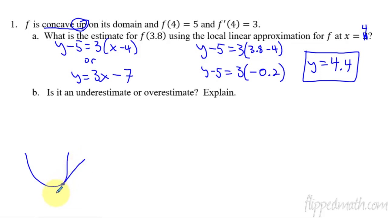
This section explores the use of the tangent line to approximate function values near the point of tangency. It explains that the tangent line can be used to approximate the function value as long as the x-value is close to the point of tangency. The paragraph also discusses the relationship between the concavity of a function and the accuracy of the tangent line approximation, noting that when the second derivative is positive, the function is concave up, and the tangent line may provide an underestimate.

15:02

🔍 Estimating Function Values Using Local Linearization

The paragraph provides an example of estimating the value of a function g(x) near the point of tangency using local linearization. It demonstrates the process of estimating g(-1.03) using the tangent line equation l(x) and shows that g(-1.03) is approximately -2.09. The importance of using an approximation symbol is emphasized, as the tangent line only equals the function value exactly at the point of tangency.

20:04

📚 Understanding Concavity and Over-Under Approximations

This section delves into the implications of a positive second derivative, indicating that the function is concave up at x = -1. It also discusses sketching the local linearization and a possible graph of y = g(x), emphasizing the importance of understanding the concavity of the function to determine whether the tangent line provides an overestimate or an underestimate.

25:07

📉 Graphical Interpretation of Local Linearization

The paragraph focuses on the graphical representation of local linearization and its relationship with the original function. It explains how the tangent line can be used to approximate the function near the point of tangency and discusses the conditions under which the tangent line gives an over or under approximation based on the concavity of the function.

30:08

🔍 Estimating with the Tangent Line at Non-Tangency Points

This section discusses the process of estimating the value of a function at a point near the point of tangency using the tangent line equation. It provides a step-by-step calculation for estimating f(2.07) using the local linearization l(x) and emphasizes the use of approximation symbols due to the proximity but not exact equality at non-tangency points.

35:09

📈 Deriving the Normal Line from the Tangent Line

The paragraph explains the concept of a normal line, which is perpendicular to the tangent line. It describes how to derive the equation of the normal line using the negative reciprocal of the tangent line's slope and the same point of tangency, highlighting the geometric relationship between the normal and tangent lines.

40:11

📚 Conclusion and Preview of Future Lessons

The final paragraph wraps up the lesson on local linearization and provides a preview of the next unit, which will explore alternative methods for finding derivatives. It signifies the end of the current topic and sets the stage for further learning in calculus.

Mindmap

Keywords

💡Local Linearization

Local linearization refers to the process of approximating a function's value near a certain point using the tangent line to the function at that point. It is integral to the theme of the video, which is to demonstrate how tangent lines can be used to approximate function values. The script uses the local linearization to estimate the value of a function near a given point, highlighting its practicality in mathematical approximations.

💡Tangent Line

A tangent line is a straight line that touches a curve at a single point without crossing it. It is central to the video's narrative, as the script explains how to derive the equation of a tangent line to a function at a specific point. The concept is exemplified through the function g(x) = -x^2 + 3x + 2, where the tangent line's equation is found to approximate the function's value at x = 2.

💡Derivative

The derivative of a function measures the rate at which the function's output changes with respect to its input. In the video, the derivative is used to find the slope of the tangent line, which is a key component of local linearization. The script demonstrates the calculation of the derivative using the limit definition, as seen with g'(x) = -2x + 3.

💡Limit Definition

The limit definition of the derivative is a fundamental concept in calculus that provides a precise way to define the derivative using limits. The video script uses this definition to calculate the derivative of the function g(x), showing the process of taking the limit as h approaches zero to find g'(x).

💡Slope

Slope is a measure of the steepness of a line, and in the context of the video, it refers to the rate of change of a function at a specific point. The script discusses how the slope of the tangent line, which is the derivative of the function at a given point, is used to approximate the function's value nearby.

💡Function Approximation

Function approximation is the process of finding a simpler function that behaves similarly to a more complex one, especially near a certain point. The video's main theme revolves around using the local linearization, or tangent line, as an approximation for the function g(x) near the point x = 2.

💡Point of Tangency

The point of tangency is the exact point where the tangent line touches the curve. The script emphasizes this concept when discussing the local linearization and the equation of the tangent line, noting that at this point, the function value and the tangent line value are the same, and the function's slope and the tangent line's slope are also the same.

💡Concave Up/Down

A function is said to be concave up if its second derivative is positive, indicating that the function is bending upwards. Conversely, it is concave down if the second derivative is negative, indicating a downward bend. The script explains how the concavity of a function affects the accuracy of the tangent line approximation and how it can indicate overestimation or underestimation.

💡Second Derivative

The second derivative of a function is the derivative of the first derivative and provides information about the function's concavity. In the video, the second derivative is used to determine whether the function is concave up or down at a given point, which in turn helps to predict whether the tangent line will overestimate or underestimate the function's value near that point.

💡Normal Line

A normal line is perpendicular to the tangent line at the point of tangency. The script briefly touches on this concept, explaining that the slope of the normal line is the negative reciprocal of the slope of the tangent line, and it passes through the same point of tangency.

Highlights

Introduction to local linearization and its use in approximating function values through tangent lines.

Derivation of the function g(x) = -x^2 + 3x + 2 using the limit definition of the derivative.

Simplification of the expression for g(x + h) and combining like terms to prepare for the limit calculation.

Finding the derivative g'(x) = -2x + 3 by evaluating the limit as h approaches zero.

Calculation of the slope of the tangent line at x = 2, resulting in g'(2) = -1.

Determination of the function value g(2) = 4 at the specified point.

Use of the point-slope form to derive the equation of the tangent line at the point (2, g(2)).

Explanation of the local linearization as an approximation method for differentiable functions.

Understanding the concept of local linearization in relation to the point of tangency and its interval.

Differentiation between a tangent line and a secant line in the context of function approximation.

Graphical representation of the tangent line and its relation to the function g(x) at x = 2.

Concept of concavity and its implications on the behavior of the tangent line relative to the function graph.

Use of the second derivative to determine if the tangent line provides an over or under approximation.

Application of local linearization to estimate the value of g(x) for x near the point of tangency.

Estimation of g(-1.03) using the local linearization and its comparison to g(-1).

Discussion on the concavity of the function g(x) and its impact on the shape of the tangent line.

Sketching the graph of the local linearization and a possible graph of y = g(x) based on the function's derivatives.

Conclusion summarizing the importance of understanding the local linearization and its applications in function approximation.

Transcripts

Browse More Related Video

Linear Approximation

Calculus AB/BC – 4.6 Approximating Values of a Function Using Local Linearity and Linearization

Linear Approximations | Using Tangent Lines to Approximate Functions

Finding The Linearization of a Function Using Tangent Line Approximations

Equation of a tangent line [IB Maths AI SL/HL]

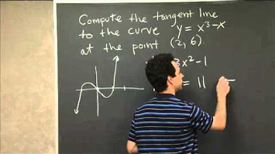
Tangent Line to a Polynomial | MIT 18.01SC Single Variable Calculus, Fall 2010

Related Tags

Local Linearization Tangent Lines Function Approximation Derivative Definition Mathematics Lesson Limit Definition Slope Calculation Graph Sketching Educational Content Calculus Concepts