Calculus AB/BC – 4.6 Approximating Values of a Function Using Local Linearity and Linearization
TLDRIn this engaging calculus lesson, Mr. Bean introduces the concept of tangent lines and their use in approximating function values. He explains that a tangent line to a function at a point can provide an approximation of the function's value at nearby points. Mr. Bean emphasizes the importance of concavity in determining whether the approximation is an overestimate or an underestimate. For a concave up function, the tangent line underestimates the function, while for a concave down function, it overestimates. Using local linear approximation, he demonstrates how to calculate the tangent line's equation and apply it to estimate function values at specific points. The lesson concludes with a practical example involving a differential equation, showcasing the power of tangent lines in approximating complex functions.
Takeaways
- 📚 The concept of a tangent line to a function at a point gives an approximation of the function's value at nearby points.
- 📈 A function that is concave up has a tangent line that lies below the function, leading to an underestimate of the function's value.
- 📉 Conversely, a function that is concave down has a tangent line that lies above the function, resulting in an overestimate of the function's value.
- 🔍 To determine if a function is concave up or down, one can look at the concavity of the function's graph, similar to the shape of a contact lens.
- 📝 The local linear approximation uses the tangent line to estimate the function's value at a point close to a given point on the graph.
- 🧮 The equation of the tangent line is derived from the point of tangency (x1, y1) and the slope of the tangent line (f'(x1)).
- 📍 For a concave up function, as you move along the tangent line away from the point of tangency, the function's value is underestimated.
- 📍 For a concave down function, as you move along the tangent line away from the point of tangency, the function's value is overestimated.
- 🔢 The process of finding the tangent line involves calculating the derivative of the function at the point of interest and using it as the slope of the tangent line.
- ✏️ The actual function's value at a point can be approximated by plugging the x-value into the equation of the tangent line.
- 🔑 Understanding the concavity of the function is crucial for determining whether the tangent line provides an overestimate or an underestimate of the function's value.
Q & A
What is the main topic of the calculus lesson?
-The main topic of the calculus lesson is tangent lines and how they can be used to approximate the value of a function at a given point.
What is the significance of concavity in the context of tangent lines?
-The concavity of a function determines whether the tangent line provides an overestimate or an underestimate of the function. If a function is concave up, the tangent line is an underestimate, and if it is concave down, the tangent line is an overestimate.
How can one identify whether a function is concave up or concave down?
-The script does not provide a method for identifying concavity within the lesson itself, but it mentions that in Unit 5.6, the teacher will show how to determine if a function is concave up or down.
What is the term used to describe the process of using a tangent line to approximate a function's value?
-The term used is 'local linear approximation', which refers to the idea that when you zoom in on a function, it appears linear and the tangent line can be used to approximate the function's value at a point.
How does the teacher demonstrate the concept of concavity?
-The teacher uses the analogy of a contact lens to explain concavity. A contact lens has a concave shape that is meant to fit the curvature of the eye. If the concavity is in the wrong direction, it can hurt when inserted.
What is the formula for the tangent line given in the script?
-The formula for the tangent line is derived from the point-slope form of a line: y - y1 = m(x - x1), where m is the slope (derivative) of the function at the point (x1, y1).
What is the estimate for the function at x = 3.8, given that the function is concave up at x = 4 with f(4) = 5 and f'(4) = 3?
-The estimate for the function at x = 3.8 using the tangent line is y = 4.4, which is an underestimate because the function is concave up.
What is the concept of a differential equation as mentioned in the script?
-A differential equation is a mathematical equation that involves a function and its derivatives. In the context of the script, it is used to find the slope of the tangent line at a particular point.
What is the initial condition given for the differential equation in the script?
-The initial condition given for the differential equation is that f(2) = 0, meaning at the point x = 2, the value of the function is 0.
How does the slope of the tangent line at a point affect the approximation of the function at nearby points?
-The slope of the tangent line at a point determines the direction and steepness of the line, which in turn affects the accuracy of the approximation. A steeper slope means the tangent line will deviate more from the function's actual curve, potentially leading to a less accurate approximation at nearby points.
What is the final estimate for the function at x = 2.2, given the differential equation and the initial condition?
-The final estimate for the function at x = 2.2, using the tangent line derived from the differential equation and the initial condition, is y = -0.4.
Outlines
📐 Understanding Tangent Lines and Their Approximations
This paragraph introduces the concept of tangent lines in calculus and their use in approximating function values. Mr. Bean explains that a tangent line to a function at a given point can provide an approximate value of the function, especially for points close to the tangent point. He uses the example of a concave up function to illustrate how the tangent line can underestimate the function's value. The paragraph also touches on the idea of concavity and how it affects the nature of the approximation—whether it's an overestimate or an underestimate.
🔍 Local Linear Approximation and Concavity
The second paragraph delves into the process of local linear approximation using tangent lines. It explains that for a concave up function, the tangent line will always be below the function, making it an underestimate. The paragraph also discusses the case of a concave down function, where the tangent line will be above the function, leading to an overestimate. The speaker provides a step-by-step example of finding a tangent line and using it to estimate the function's value at a nearby point, highlighting the importance of staying close to the tangent point for a better approximation.
🧮 Applying Tangent Line Approximation with Differential Equations
The final paragraph presents a more complex scenario involving a differential equation. It explains that even without knowing the original function, one can still use the tangent line to approximate function values. The speaker demonstrates how to find the slope of the tangent line using the derivative and then use this to estimate the function's value at a specific point. The paragraph emphasizes that without information on the function's concavity, it's not possible to determine whether the approximation is an underestimate or an overestimate. It concludes with an encouragement to practice these concepts in the mastery check.
Mindmap
Keywords
💡Tangent line
💡Concavity
💡Local linear approximation
💡Derivative
💡Underestimate and Overestimate
💡Differential equation
💡Initial condition
💡Anti-derivative
💡Concave up and concave down
💡Mastery check
💡Approximation
Highlights
The lesson discusses tangent lines and how they can be used to approximate function values at points close to a given point x=a.
The concept of concavity is introduced, explaining how it affects whether the tangent line is an overestimate or underestimate of the function.
A function that is concave up will have a tangent line that underestimates the function value, while a concave down function will have a tangent line that overestimates it.
The process of finding the equation of a tangent line at a point (x1, y1) is demonstrated, using the point and the derivative (slope) at that point.
An example is worked through where the function f is concave up, f(4)=5, and f'(4)=3. The tangent line is used to estimate f(3.8), resulting in an underestimate of 4.4.
For a concave down function, the tangent line will overestimate the function value. An example is shown where f(1)=1, f'(1)=-1, and the tangent line overestimates f(1.1) as 0.8.
A differential equation is provided, and the process of finding the tangent line at a point (2,0) is shown, resulting in an estimate of -0.4 for the function value at x=2.2.
The lesson emphasizes that the tangent line provides a local linear approximation of the function near a given point.
The importance of staying close to the point of tangency for a better approximation is highlighted.
The concept of concavity is related to the shape of a contact lens, with concave up resembling a lens that opens up like a ball.
A method to determine if a function is concave up or down will be covered in a later lesson, so students do not need to worry about it for now.
The lesson provides a clear, step-by-step approach to using tangent lines to approximate function values, making it accessible to students.
The use of the tangent line equation in different forms (y-y1 = m(x-x1) or y = mx + b) is demonstrated, showing flexibility in calculations.
The lesson includes a mastery check to reinforce the concepts and give students a chance to practice.
The instructor uses humor and relatable analogies (e.g. contact lens) to make the material more engaging and easier to understand.
The lesson provides a solid foundation for more advanced calculus topics like anti-derivatives that will be covered later.
The instructor emphasizes the importance of understanding the concavity of a function and how it affects the accuracy of the tangent line approximation.
Transcripts
Browse More Related Video
AP Calculus AB: Lesson 2.6 Tangent Line Approximations
Linear Approximation
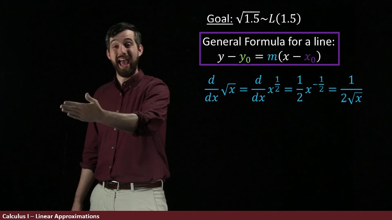
Linear Approximations | Using Tangent Lines to Approximate Functions
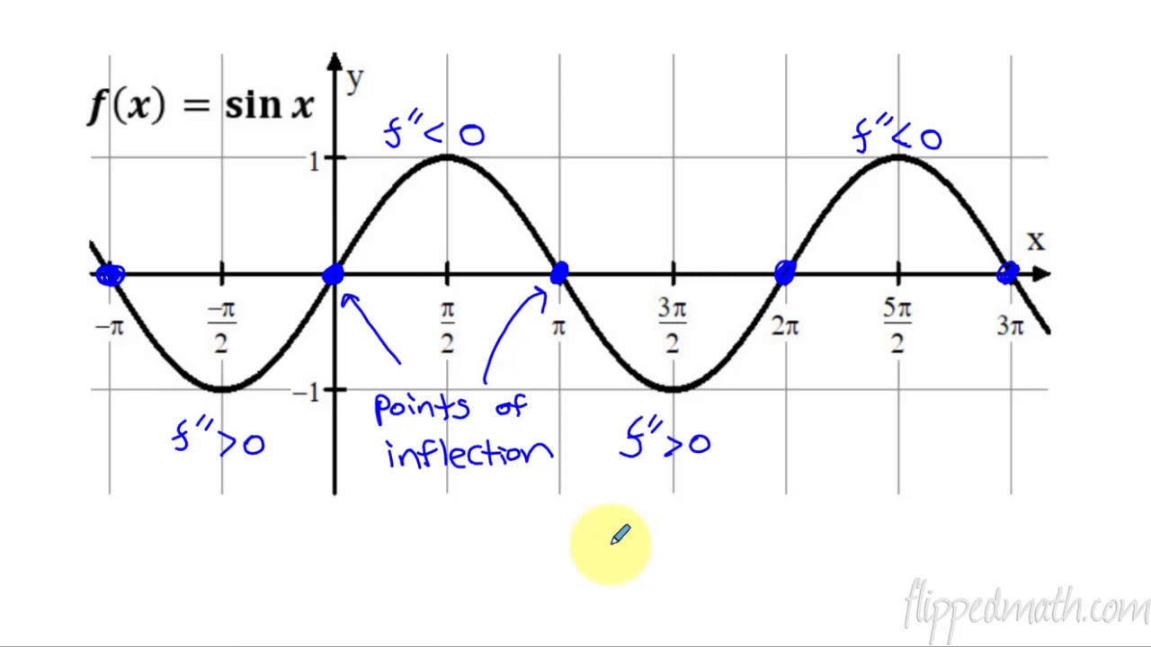
Calculus AB/BC – 5.6 Determining Concavity of Functions over Their Domains
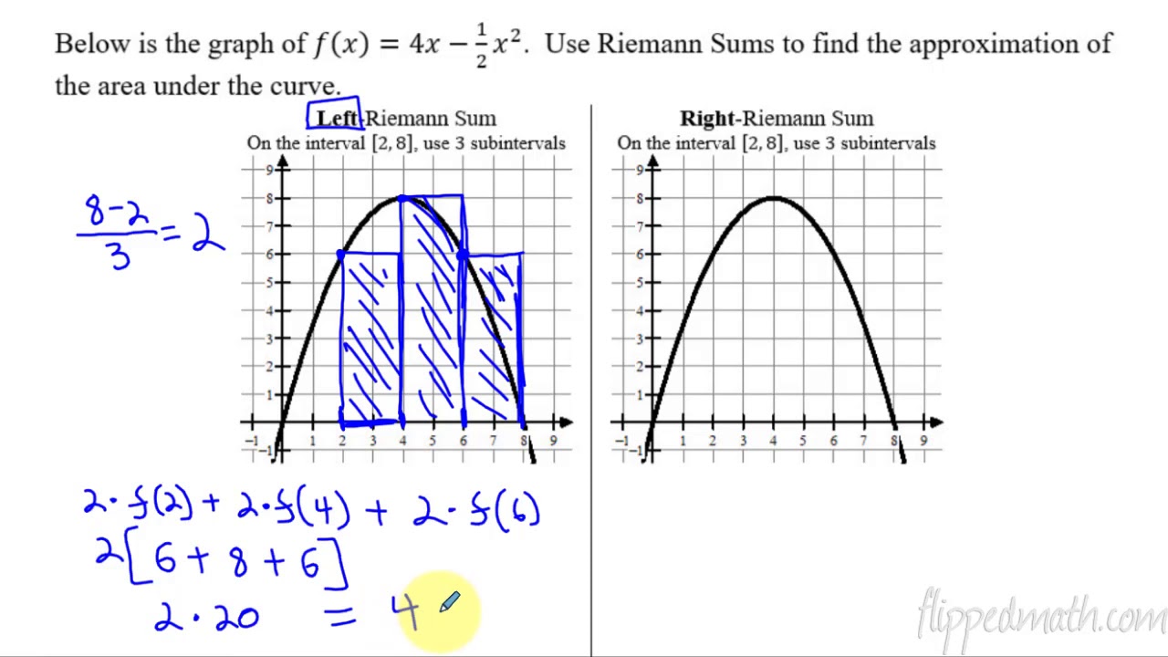
Calculus AB/BC – 6.2 Approximating Areas with Riemann Sums
2022 AP Calculus AB Exam FRQ #5
5.0 / 5 (0 votes)
Thanks for rating: