Probability density functions | Probability and Statistics | Khan Academy
TLDRThis video script introduces the concept of random variables, distinguishing between discrete and continuous types. Discrete variables have a finite number of outcomes, often integers, while continuous variables can take an infinite number of values. The script uses the example of the exact amount of rain tomorrow to illustrate continuous variables and their probability density functions. It explains that the probability of an exact value is essentially zero, emphasizing the importance of calculating areas under the curve to determine probabilities for ranges of values. The video concludes with the fundamental principle that the sum of all probabilities or areas under the curve must equal one, setting the stage for the next topic: expected value.
Takeaways
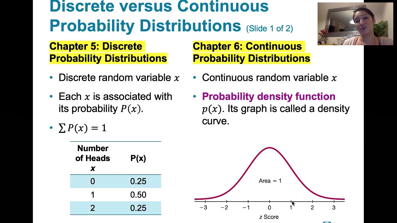
- 📚 The video introduces the concept of random variables, distinguishing between discrete and continuous types.
- 🔢 Discrete random variables have a finite number of possible outcomes, which are not necessarily integers.
- 🌊 Continuous random variables can take an infinite number of values, such as the exact amount of rain in an example given.
- 📈 The probability distribution function for continuous variables is represented by a probability density function (PDF), which is visualized as a curve.
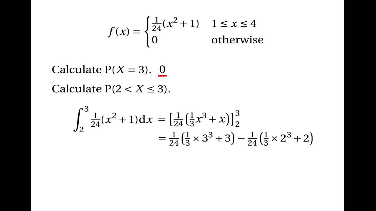
- 🎯 The probability of a continuous random variable taking an exact value is essentially zero, due to the infinite precision required.
- 📏 To find the probability for a continuous variable, one must consider intervals and calculate the area under the PDF curve for that range.
- ∫ The area under the PDF curve is found using definite integrals from calculus, which represent the probability of an event occurring within a certain interval.
- 🌀 The entire area under the PDF curve must sum up to 1, representing the certainty that one of the possible outcomes will occur.
- 💡 Understanding continuous random variables involves thinking about probabilities in terms of intervals and areas rather than exact values.
- 🧩 Both discrete and continuous probability distributions must have their probabilities sum up to 1, ensuring all possible outcomes are accounted for.
- 🚀 The video concludes with a teaser for the next topic, which will be the concept of expected value.
Q & A
What is the main difference between discrete and continuous random variables?
-Discrete random variables take on a finite number of values, often integers, whereas continuous random variables can take on an infinite number of values within a range.
Why are continuous random variables often represented by capital letters?
-There is no strict rule, but it is a common convention to use capital letters for continuous random variables, such as Y in the example given.
What is a probability density function (PDF) and how does it relate to continuous random variables?
-A probability density function is a function that describes the likelihood of a continuous random variable taking on a particular value. The area under the curve of the PDF between two points represents the probability of the random variable falling within that interval.
Why is the probability of a continuous random variable being exactly a certain value typically 0?
-Because continuous random variables can take on an infinite number of values, the chance of it being exactly a specific value, to an infinite decimal point, is essentially 0 due to the precision required.
How can we calculate the probability of a continuous random variable falling within a certain range?
-We calculate it by finding the area under the probability density function for that range, which is done using the definite integral of the PDF from one boundary to the other.
What is the significance of the area under the entire probability density function being equal to 1?
-The area under the entire PDF being equal to 1 ensures that the sum of all possible probabilities of the random variable occurring is 100%, which is a fundamental property of probability distributions.
What is the relationship between the sum of probabilities in a discrete probability distribution and the area under the PDF in a continuous distribution?
-Both must equal 1. In a discrete distribution, the sum of all individual probabilities must add up to 1. In a continuous distribution, the area under the PDF from the lowest to the highest value must also equal 1.
Why is it important to understand the concept of 'tolerance' when dealing with continuous random variables?
-Tolerance is important because it allows us to define intervals within which the random variable is likely to fall, making it possible to calculate meaningful probabilities instead of dealing with the theoretical 0 probability of exact values.
Can you provide an example of how to calculate the probability of a continuous random variable being within a specific range?
-Yes, if you want to find the probability that a continuous random variable Y is between 1.9 and 2.1, you would calculate the definite integral of the PDF from x=1.9 to x=2.1.
What is the concept that will be introduced in the next video after the one described in the transcript?
-The next video will introduce the concept of expected value, which is a key measure in probability theory and statistics.
Outlines
📊 Understanding Discrete and Continuous Random Variables
The script begins with a recap of the concepts introduced in the previous video, focusing on random variables. It differentiates between discrete and continuous random variables, explaining that discrete variables have a finite number of outcomes, which are not necessarily integers. The video uses the example of the amount of rain tomorrow to illustrate a continuous random variable, which can take an infinite number of values. The instructor emphasizes that the probability of a continuous variable taking an exact value is essentially zero, because in reality, measurements can never be perfectly precise. The concept of a probability density function (PDF) is introduced, with a visual representation that peaks at 0.5 inches of rain, to help viewers understand how continuous variables are represented and interpreted.
📚 Calculating Probabilities for Continuous Variables
This paragraph delves deeper into the concept of continuous random variables, explaining that the probability of a variable taking an exact value is zero due to the infinitesimally small chance of a measurement being perfectly precise. The instructor introduces the idea of calculating probabilities for ranges of values, which is done by finding the area under the probability density function for a given interval. The use of calculus, specifically definite integrals, is highlighted as the mathematical tool to calculate these areas. The importance of the entire area under the curve summing up to 1 is emphasized, which corresponds to a 100% chance that one of the possible outcomes will occur. The video also touches on the concept of discrete probability distributions, where the sum of probabilities for all possible outcomes must equal 1, using a coin toss as an example. The script concludes with a teaser for the next video, which will cover the concept of expected value.
Mindmap
Keywords
💡Random Variable
💡Discrete Random Variable
💡Continuous Random Variable
💡Probability Distribution Function
💡Probability Density Function
💡Exact Value Probability
💡Area Under the Curve
💡Definite Integral
💡Tolerance
💡Sum of Probabilities
Highlights
Introduction to the concept of random variables.
Differentiation between discrete and continuous random variables.
Explanation that discrete random variables have a finite number of values, not necessarily integers.
Continuous random variables can take on an infinite number of values.
Use of capital letters to denote continuous random variables, exemplified by variable Y.
Example of a continuous random variable: the exact amount of rain tomorrow.
Drawing of a probability density function to represent continuous random variables.
Clarification that the probability of an exact value for a continuous variable is essentially zero.
Logical reasoning behind why it's impossible to have an exact measurement of continuous variables.
Interpretation of probability in terms of intervals and areas under the curve.
Calculation of probability as the definite integral of the probability density function.
Explanation of how to find the probability of a range of values for a continuous variable.
The importance of the total area under the curve summing up to 1 for probability distributions.
Application of the same principle to discrete probability distributions.
Illustration of a discrete probability distribution with a coin flip example.
Emphasis on the sum of probabilities equating to 1 for both discrete and continuous distributions.
Upcoming introduction to the concept of expected value in the next video.
Transcripts
Browse More Related Video

Discrete and continuous random variables | Probability and Statistics | Khan Academy
Continuous Random Variables: Probability Density Functions
6.1.1 The Standard Normal Distribution - Discrete and Continuous Probability Distributions
Introduction to Discrete Random Variables and Discrete Probability Distributions

Elementary Statistics - Chapter 5 Probability Distributions Part 1
5.1.2 Discrete Probability Distributions - Probability Distributions and Probability Histograms
5.0 / 5 (0 votes)
Thanks for rating: