6.1.1 The Standard Normal Distribution - Discrete and Continuous Probability Distributions
TLDRThis educational video script delves into the comparison between discrete and continuous probability distributions. It explains discrete random variables with countable outcomes, like coin tosses, and continuous variables with uncountable outcomes, such as body temperatures. The script clarifies the concept of the probability density function (PDF) and its integral role in defining the probability for ranges of values in continuous distributions. It also contrasts discrete probability histograms with the density curves of continuous distributions, emphasizing the total area under the curve equating to one, representing total probability. The script encourages viewers to explore further with a recommended video on the nuances of probability density functions.
Takeaways
- 📚 The video discusses learning outcome number one of lesson 6.1, focusing on comparing and contrasting discrete and continuous probability distributions.
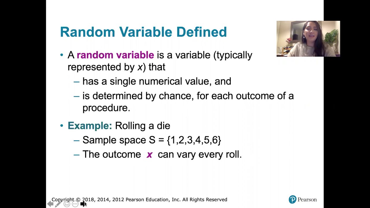
- 📈 Discrete random variables have a finite or infinite but countable set of values, such as the number of coin tosses before getting heads.
- 📊 Continuous random variables have an uncountable set of values over a range, like body temperatures, which can take any value within a certain range.
- 📝 The probability density function (PDF) is a key concept for continuous distributions, differentiating it from discrete distributions where each value has an associated probability.
- 📉 The graph of a discrete random variable on a number line consists of individual points, while continuous variables are represented by a curve, indicating a range of possible values.
- 🔢 In discrete distributions, the sum of probabilities must equal one, as one of the possible outcomes must occur. In contrast, the area under the continuous distribution curve, representing probabilities, must also equal one.
- 📋 The video script revisits the definitions and examples from previous chapters, such as summarizing data in tables and calculating sample mean and standard deviation.
- 🎲 Chapter five integrates concepts from previous chapters, combining data organization and probability to create a theoretical model of expected results for discrete distributions.
- 🌐 The script emphasizes the difference between sample statistics and population parameters, highlighting that chapter five deals with theoretical probabilities for the entire population.
- 📝 The probability histogram is used to visualize discrete distributions, where the height of each bar represents the probability of a specific outcome.
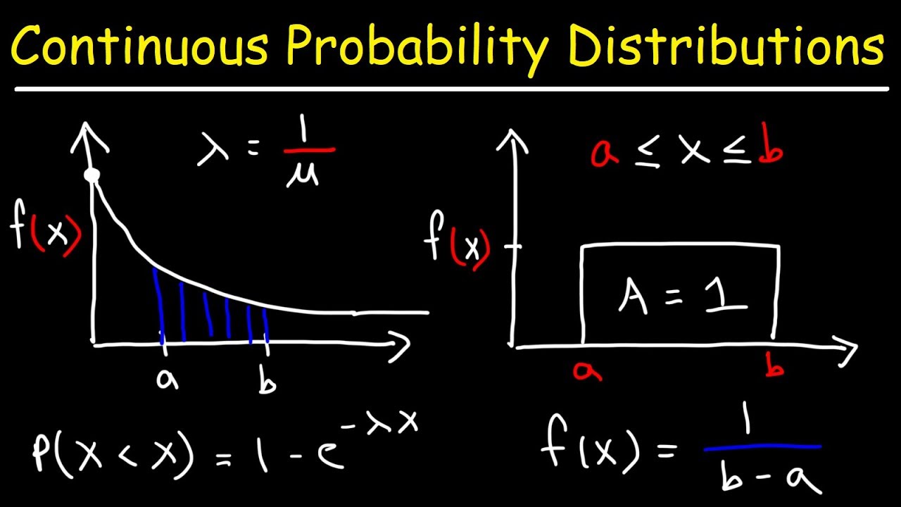
- 📉 For continuous distributions, the area under the curve of the PDF between two points represents the probability of the random variable falling within that range, such as the probability of a man's height being between certain measurements.
Q & A
What is the main focus of the video script?
-The video script focuses on comparing and contrasting discrete and continuous probability distributions, explaining the properties of continuous probability distributions, defining the probability density function, and its relationship to probability.
What is a discrete random variable?
-A discrete random variable has a collection of values that is finite or infinite but countable, such as the number of coin tosses before getting heads.
How is a discrete random variable represented on a number line?
-A discrete random variable is represented on a number line as a series of distinct points, such as 2, 4, 6, and 8, without any values in between.
What is an example of a discrete random variable?
-An example of a discrete random variable is the count of the number of movie patrons at a movie theater, which increments by one each time someone enters.
What is a continuous random variable?
-A continuous random variable has infinitely many values that extend over a range and is not countable, such as body temperatures.
How does the value range of a continuous random variable differ from a discrete random variable?
-The value range of a continuous random variable is uncountably infinite and covers a range of values, unlike a discrete random variable which has countable, distinct values.
What is the probability density function (PDF) in the context of continuous probability distributions?
-The probability density function (PDF) is a function that describes the likelihood of the random variable taking on a particular value, with the total area under the curve equaling one.
How is the probability of a continuous random variable found?
-The probability of a continuous random variable is found by calculating the area under the probability density function (PDF) curve between two specified values.
What is the difference between a probability histogram for discrete distributions and a density curve for continuous distributions?
-A probability histogram for discrete distributions shows the sum of probabilities as the heights of bars, while a density curve for continuous distributions shows the area under the curve representing probabilities for ranges of values.
Why is the area under the PDF curve important in continuous probability distributions?
-The area under the PDF curve is important because it represents the probability of the random variable falling within a certain range of values, and the total area under the curve must equal one.
What does the video script suggest for further understanding of probability density functions?
-The video script suggests watching a video by Grant Sanderson from Three Blue One Brown, titled 'Why a probability of zero does not mean an event is impossible,' for a better understanding of probability density functions.
Outlines
📊 Discrete vs. Continuous Probability Distributions
This paragraph introduces the learning outcome of comparing discrete and continuous probability distributions. It explains the properties of continuous distributions and the concept of the probability density function (PDF). The paragraph also revisits the definitions of discrete and continuous random variables, giving examples like coin tosses and body temperatures. The difference between the countable outcomes of discrete variables and the uncountable range of continuous variables is highlighted, along with the graphical representation of these variables on a number line.
📈 Summarizing Data and Probability in Discrete Distributions
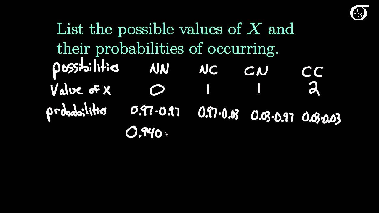
The second paragraph delves into the process of summarizing and organizing data using frequency distributions and histograms, as well as calculating sample mean and standard deviation. It contrasts this with the theoretical probabilities associated with events like coin tosses, which are part of discrete probability distributions. The paragraph explains how chapter five combined data organization with probability theory to create a model of expected results, using the example of tossing a coin twice and the associated probabilities for getting zero, one, or two heads.
📚 Transition from Discrete to Continuous Probability Distributions
This paragraph transitions from discussing discrete random variables and their associated probabilities to the concept of continuous random variables and their probability density functions. It emphasizes the shift from individual probabilities summing to one to the total area under the density curve equating to one. The paragraph also introduces the idea of contrasting discrete and continuous distributions, setting the stage for the detailed exploration of continuous distributions in chapter six.
📉 Understanding Continuous Probability Density Functions
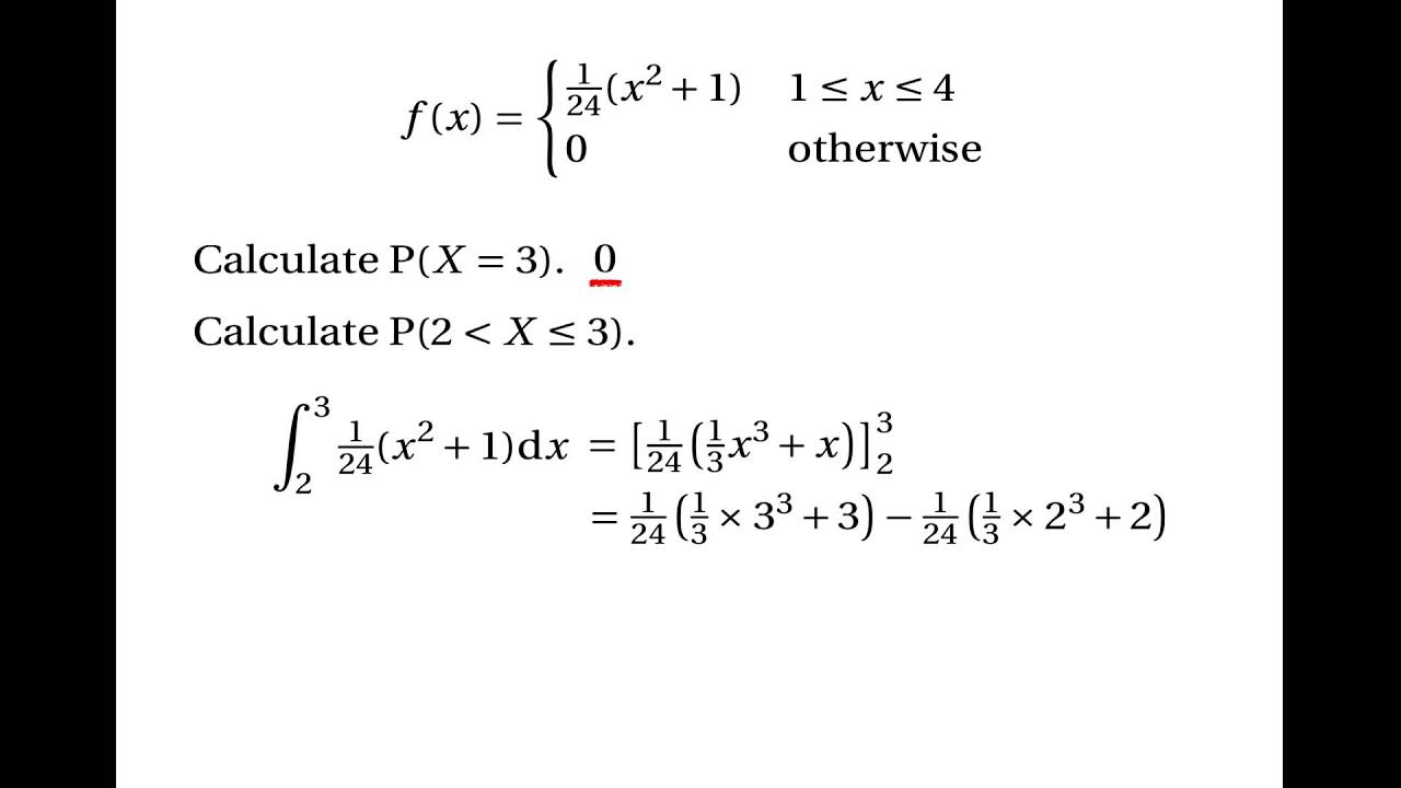
The fourth paragraph focuses on the probability density function (PDF) for continuous random variables, explaining that it describes the distribution over a range of values rather than individual outcomes. It clarifies that the PDF, denoted as p(x), provides the probability per change in x, not the probability of x being a specific value. The concept of finding the probability for a range of values by calculating the area under the curve is introduced, with an example of men's height distribution and the probability of a man being taller than 72 inches.
🔍 Probabilities of Zero and the Nature of Continuous Variables
The final paragraph addresses the misconception that a probability of zero means an event is impossible, especially in the context of continuous variables. It explains that for continuous distributions, probabilities are associated with ranges of values, not specific outcomes. The paragraph encourages viewers to watch a video by Grant Sanderson from '3Blue1Brown' for a deeper understanding of probability density functions and the significance of areas under the curve in continuous distributions.
Mindmap
Keywords
💡Discrete Random Variable
💡Continuous Random Variable
💡Probability Density Function (PDF)
💡Discrete Probability Distribution
💡Continuous Probability Distribution
💡Density Curve
💡Sample Mean and Sample Standard Deviation
💡Population Mean and Population Standard Deviation
💡Frequency Distribution
💡Probability Histogram
💡Theoretical Model
Highlights
The video discusses the comparison and contrast between discrete and continuous probability distributions.
It aims to teach the properties of continuous probability distributions and define the probability density function.
Discrete random variables have finite or infinite but countable values, like the number of coin tosses before getting heads.
Continuous random variables have infinitely many values over a range, such as body temperatures.
Graphing discrete random variables results in points on a number line, unlike continuous variables.
Examples of discrete random variables include the count of movie patrons at a theater.
Continuous random variables, like battery voltage, extend over a range with infinitely many values.
Chapter five combined data summarization with probability to model expected results.
In chapter five, discrete probability distributions were used to model outcomes like coin tosses.
Chapter six introduces continuous probability distributions, contrasting with the discrete approach.
The probability density function (PDF) is central to understanding continuous probability distributions.
The total area under the PDF curve represents the total probability, which must equal one.
The probability for a range of values in a continuous distribution is found by calculating the area under the curve.
The video explains the difference between discrete and continuous probability distributions using histograms and density curves.
The probability density function does not give the probability for a single value but per change in value.
A practical example of a continuous random variable is the normally distributed heights of men with a mean of 68.6 inches.
The video recommends watching another video by Grant Sanderson for a deeper understanding of probability density functions.
The concept that a probability of zero does not mean an event is impossible is clarified for continuous variables.
Transcripts
Browse More Related Video
Continuous Random Variables: Probability Density Functions

Session 40 - Probability Distribution Functions - PDF, PMF & CDF | DSMP 2023
Probability density functions | Probability and Statistics | Khan Academy
5.1.1 Discrete Probability Distributions - Discrete and Continuous Random Variables
Introduction to Discrete Random Variables and Discrete Probability Distributions
Continuous Probability Distributions - Basic Introduction
5.0 / 5 (0 votes)
Thanks for rating: