Introduction to Discrete Random Variables and Discrete Probability Distributions
TLDRThe video introduces discrete random variables, using the example of rolling a die four times to count the number of sixes. It explains that a random variable takes on numerical values based on chance and can be either discrete or continuous. Discrete random variables have countable possible values, like the number of sixes in dice rolls, while continuous random variables can take any value within an interval, like water level in a container. The video also illustrates the probability distribution of discrete random variables and contrasts it with continuous distributions.
Takeaways
- 🎲 The concept of a discrete random variable is introduced with an example of rolling a die multiple times and counting the number of sixes.
- 📊 Discrete random variables can take on a countable number of possible values, such as the outcomes of rolling a die, which are 0, 1, 2, 3, or 4 sixes.
- 🔢 Random variables are categorized as either discrete or continuous, with discrete variables having distinct possible values and continuous variables having a range of possible values.
- 🌐 Discrete random variables are not always count data; they can also take on specific values like 1.5, 2.5, and 3.5, which are still considered discrete.
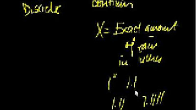
- 💧 Continuous random variables, in contrast, can take any value within an interval, such as the amount of water in a container ranging from 0 to 2 liters.
- 📚 Examples of discrete random variables include the number of lottery tickets purchased until the first win and the number of courses a university student is taking.
- ⏱ Examples of continuous random variables include the time until a new website gets its first hit and the height of an adult Canadian male.
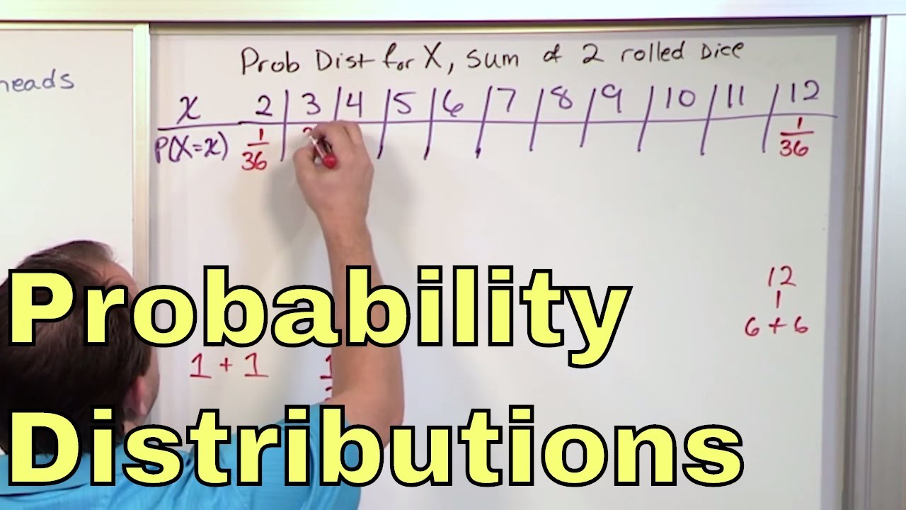
- 👥 A probability distribution for a random variable lists all possible values and their associated probabilities, such as the number of adults under correctional supervision in a sample.
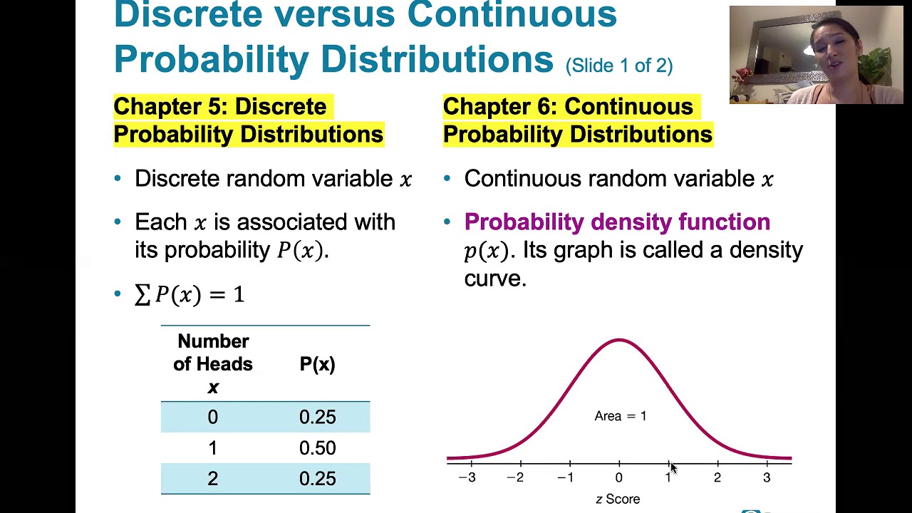
- 📉 Discrete probability distributions must satisfy certain conditions: probabilities must be between 0 and 1, and the sum of all probabilities must equal 1.
- 📈 Visual representations of discrete probability distributions can help in understanding the likelihood of different outcomes, as shown by plotting the values and their probabilities.
- 📊 The script contrasts discrete and continuous probability distributions, highlighting the difference in how they are represented and the nature of the values they can take.
Q & A
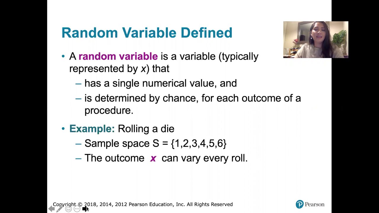
What is a discrete random variable?
-A discrete random variable is a variable that can take on a countable number of possible values, often from a set of distinct values, according to some sort of chance process involving randomness.
How is a discrete random variable different from a continuous random variable?
-A discrete random variable can only take on a countable number of distinct values, whereas a continuous random variable can take on any value within an interval, representing an infinite number of possible values.
What is an example of a discrete random variable that is not a count?
-An example of a discrete random variable that is not a count is one that takes on the values 1.5, 2.5, and 3.5. These values are distinct and countable, but they do not represent a count of items.
Can you explain the concept of a probability distribution for a random variable?
-A probability distribution for a random variable is a listing, formula, or graphic representation of all possible values of the variable and their respective probabilities of occurring.
What are the conditions that all discrete probability distributions must satisfy?
-All discrete probability distributions must satisfy the conditions that each probability p(x) must be between 0 and 1, and the sum of all probabilities must equal 1.
How many possible values can a discrete random variable take on in the example of rolling a die four times and recording the number of sixes?
-In the example of rolling a die four times, the discrete random variable (number of sixes) can take on 5 possible values: 0, 1, 2, 3, or 4 sixes.
What is an example of a continuous random variable as described in the script?
-An example of a continuous random variable given in the script is the amount of water in a container with a maximum capacity of 2 liters, which can take on any value between 0 and 2 liters.
What is the probability that a randomly sampled US adult is under correctional supervision, according to the example in the script?
-According to the example in the script, the probability that a randomly sampled US adult is under correctional supervision is 3%, or 0.03.
How are the probabilities of the possible outcomes calculated for the example of sampling two US adults?
-The probabilities are calculated by considering the independent and random sampling of two adults. The probabilities are found by multiplying the individual probabilities of each outcome, such as (0.97 * 0.97) for both not being under supervision, (0.97 * 0.03) for the first not being under supervision and the second being, and so on.
What is the purpose of plotting a discrete probability distribution?
-Plotting a discrete probability distribution helps to visually represent the likelihood of each possible outcome, showing the relative probabilities of the random variable taking on different values.
How does the visual representation of a continuous probability distribution differ from that of a discrete one?
-A continuous probability distribution is represented by a smooth curve, indicating the range of possible values without distinct jumps between values, as opposed to a discrete distribution which shows distinct jumps between countable values.
Outlines
🎲 Introduction to Discrete Random Variables
This section introduces the concept of discrete random variables using the example of rolling a die four times and recording the number of sixes. It explains that a discrete random variable takes on numerical values based on a chance process and can have a countable number of possible values. The difference between discrete and continuous random variables is highlighted, with discrete variables having distinct possible values and continuous variables taking any value within an interval.
🔢 Probabilities of Random Variables
This section delves into the representation of random variables, often denoted by capital letters like X, Y, or Z. It explores possible values and their probabilities using the example of US adults under correctional supervision. By calculating probabilities for different scenarios (e.g., none, one, or both adults under supervision), it demonstrates how to create a probability distribution for a random variable and the conditions that must be met: probabilities lying between 0 and 1, and their sum equating to 1.
📊 Visualizing Probability Distributions
The final section contrasts discrete and continuous probability distributions. Discrete distributions have distinct jumps between values, as seen in the example of X representing the number of adults under correctional supervision. Continuous distributions, such as the heights of Canadian males, are represented by smooth curves without discrete jumps. The section emphasizes the need to handle these types of distributions differently and visualizes them to better understand their behavior.
Mindmap
Keywords
💡Discrete Random Variable
💡Continuous Random Variable
💡Probability Distribution
💡Probability
💡Random Variable
💡Countable
💡Independence
💡Sample
💡Distribution Curve
💡Expected Value
Highlights
Introduction to discrete random variables and their role in chance processes.
Explanation of a random variable as a numerical outcome of a random process.
Difference between discrete and continuous random variables in terms of the number of possible values.
Discrete random variables can have a countable number of possible values, such as the outcomes of rolling a die.
Continuous random variables can take any value within an interval, unlike discrete variables with distinct values.
Examples of discrete random variables, including the number of lottery tickets until a winning ticket is found.
Examples of continuous random variables, such as the time until a website gets its first hit.
The concept of a probability distribution for a random variable, listing all possible values and their probabilities.
How to calculate the probabilities of different outcomes for a discrete random variable, using the example of sampling US adults under correctional supervision.
The importance of ensuring that probabilities for a discrete distribution lie between 0 and 1 and sum up to 1.
Visual representation of a discrete probability distribution, showing the difference from a continuous distribution.
The practical application of understanding discrete and continuous random variables in various real-world scenarios.
The use of capital letters to represent random variables and the notation p(x) for the probability of a random variable taking a specific value.
Explanation of how to represent the probability of a random variable taking on a value using p(x), where x is the value.
The process of creating a probability distribution for a discrete random variable, as demonstrated with the example of US adults under correctional supervision.
The conditions that all discrete probability distributions must satisfy, including the range of probabilities and their sum.
Contrasting the discrete jumps in a discrete probability distribution with the smooth curve of a continuous distribution.
The significance of understanding the difference in handling discrete and continuous probability distributions in statistical analysis.
Transcripts
Browse More Related Video
5.1.1 Discrete Probability Distributions - Discrete and Continuous Random Variables

Discrete and continuous random variables | Probability and Statistics | Khan Academy
Introduction to Random Variables

Probability density functions | Probability and Statistics | Khan Academy
6.1.1 The Standard Normal Distribution - Discrete and Continuous Probability Distributions
02 - Random Variables and Discrete Probability Distributions
5.0 / 5 (0 votes)
Thanks for rating: