5.1.2 Discrete Probability Distributions - Probability Distributions and Probability Histograms
TLDRThis video script delves into the concept of probability distributions, explaining how they assign probabilities to each value of a random variable, which can be represented in tables, formulas, or graphs like probability histograms. It outlines three key conditions for a valid distribution: the variable must be numerical, the sum of probabilities must equal one, and each probability must lie between zero and one. The script uses examples to illustrate these concepts, including distinguishing between discrete and continuous variables and the importance of not rounding probabilities to zero. It also introduces the idea of representing distributions with formulas, previewing a deeper exploration in upcoming lessons.
Takeaways
- 📊 A probability distribution assigns probabilities to each value of a random variable and can be represented in tables, formulas, or probability histograms.
- 🔢 Probability distributions must satisfy three conditions: existence of a numerical random variable, sum of probabilities equaling 1, and each individual probability being between 0 and 1 inclusive.
- 🚫 If a table contains categories, it does not represent a probability distribution because random variables are numerical, not categorical.
- 🔍 Rounding errors can occur when summing probabilities, but the sum should ideally be 1, indicating all possible outcomes are accounted for.
- 💡 'Zero plus' in a probability table indicates a very small probability that is positive but typically rounded to zero, signifying an event is extremely unlikely but not impossible.
- 🧬 The example of X-linked genetic disorders in children demonstrates how a probability distribution can be used to represent the likelihood of different outcomes.
- 📊 To determine if a table represents a probability distribution, check if it meets the conditions for a random variable, the sum of probabilities, and the range of individual probabilities.
- 📈 Probability histograms are a graphical representation of probability distributions, with the area of bars corresponding to probabilities when the bars are one unit wide.
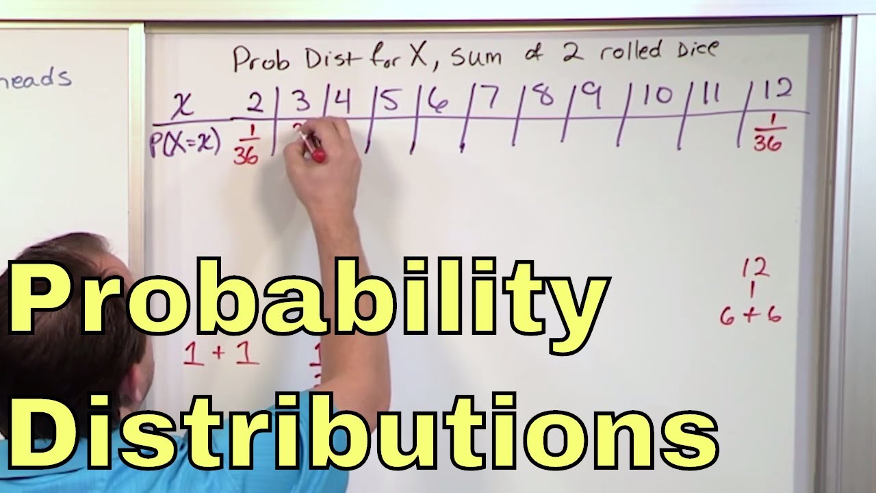
- 🎲 The formula for the number of heads in two coin tosses illustrates how probabilities can be calculated using mathematical expressions and is related to binomial distributions.
- 📉 A table based on categorical data, such as common job interview mistakes, does not represent a probability distribution because it does not meet the condition of having a numerical random variable.
- 📚 Understanding the mean, variance, and standard deviation of a probability distribution is crucial for further statistical analysis and will be discussed in subsequent lessons.
Q & A
What is a probability distribution?
-A probability distribution gives the probability for each value of a random variable. It can be expressed in various forms such as a table, a formula, or a graph called a probability histogram.
What are the three conditions that a probability distribution must satisfy?
-The three conditions are: 1) There must be a random variable x, which is numerical, not categorical. 2) The sum of the probabilities for all possible values of x must equal 1, allowing for slight rounding errors. 3) The probability for each value of x must be between zero and one, inclusive.
What does 'zero plus' represent in a probability table?
-'Zero plus' in a probability table represents a probability value that is positive but very small, typically rounded to zero but not actually zero, indicating an event that is extremely unlikely but not impossible.
How can you determine if a table represents a probability distribution?
-To determine if a table represents a probability distribution, check if it meets the three conditions: 1) x is a numerical random variable, 2) the sum of probabilities equals 1, and 3) each probability is between zero and one.
What is the difference between a discrete and a continuous random variable?
-A discrete random variable takes on a finite or countably infinite number of values, whereas a continuous random variable can take on any value within an interval or set of intervals.
How is a probability histogram different from a relative frequency histogram?
-A probability histogram is similar to a relative frequency histogram, but instead of frequencies or relative frequencies on the vertical axis, it has probabilities.
What is the relationship between the area of the bars in a probability histogram and the probabilities of the random variable?
-In a probability histogram, the area of each bar (length times height) represents the probability of the corresponding value of the random variable, especially when the bars are one unit wide.
Can probability distributions be described with formulas?
-Yes, probability distributions can often be described with formulas, which can be used to calculate the probability for different values of the random variable.
How is the formula for the number of heads in two coin tosses derived?
-The formula is derived from the principles of binomial distributions and is given by (1/2) * (2 - x)! * x!, where x can be 0, 1, or 2. This formula will be discussed in more detail in the next lesson.
Why is the table of job interview mistakes not a probability distribution?
-The table of job interview mistakes is not a probability distribution because it does not meet the condition that x must be a numerical random variable (it's categorical), and the sum of the probabilities does not equal 1.
What will be discussed in the next part of the lesson regarding probability distributions?
-In the next part of the lesson, the focus will be on finding the mean, variance, and standard deviation given a probability distribution.
Outlines
📊 Understanding Probability Distributions
This paragraph delves into the concept of probability distributions, explaining that they assign probabilities to every possible outcome of a random variable. It highlights the three key conditions that a distribution must meet: the presence of a numerical random variable, the sum of probabilities equating to 1, and each individual probability being between 0 and 1 inclusive. The paragraph also clarifies the distinction between numerical and categorical data, using an example of a genetic disorder inheritance to illustrate a valid probability distribution. It further discusses the representation of extremely small probabilities as 'zero plus' to indicate a non-zero chance of an event occurring.
📈 Visualizing Probability Distributions with Histograms
This section introduces the visualization of probability distributions through probability histograms, which are similar to relative frequency histograms but with probabilities on the vertical axis. The example of coin tosses for heads is used to demonstrate how probabilities are represented graphically, with the area of the bars in the histogram corresponding to the probability of each outcome. The importance of the area representing probability is emphasized, setting the stage for further discussions in chapter six. The paragraph also touches on the representation of probability distributions using formulas, using the binomial distribution of coin tosses as an example to show how probabilities can be calculated and verified with a formula.
🔍 Evaluating Data for Probability Distributions
The final paragraph examines the criteria for determining whether a set of data represents a probability distribution. It uses a table of job interview mistakes and their associated probabilities to illustrate the process of validation. The paragraph points out that the data fails to meet the criteria for a probability distribution due to the categorical nature of the data and the sum of probabilities exceeding 1. It emphasizes the importance of understanding the meaning behind the numbers in a dataset before it can be interpreted correctly, and concludes with a transition to future topics on calculating mean, variance, and standard deviation from a given probability distribution.
Mindmap
Keywords
💡Probability Distribution
💡Random Variable
💡Probability Histogram
💡Conditions for Probability Distributions
💡Categorical Data
💡Discrete Random Variable
💡Continuous Random Variable
💡Zero Plus (0+)
💡Sample Space
💡Binomial Distribution
Highlights
Definition of a probability distribution: It provides the probability for each value of a random variable and can be expressed in various forms such as a table, formula, or probability histogram.
Three conditions for probability distributions: 1) Existence of a numerical random variable x, 2) Sum of probabilities equals 1, and 3) Each probability value is between 0 and 1 inclusive.
Explanation of rounding errors in probability tables where the sum might slightly deviate from 1 due to rounding but should ideally equal 1.
Clarification on the use of 'zero plus' to represent very small probabilities that are not exactly zero but are extremely unlikely.
Example of a probability distribution in a genetic disorder scenario, illustrating how the number of children inheriting a disorder is a discrete random variable.
Determination of whether a table represents a probability distribution by checking if it satisfies the three conditions, including the sum of probabilities equaling 1.
Differentiation between discrete and continuous random variables based on the finite number of possible values.
Introduction to probability histograms as a visual representation of probability distributions, differing from frequency histograms by showing probabilities instead of frequencies.
Illustration of a probability histogram for the number of heads when tossing a coin twice, demonstrating how the area under the bars represents the probability.
Explanation of how the area of rectangles in a histogram corresponds to the probability when the random variable values are integers.
Presentation of a formula for calculating the probability of getting a certain number of heads in two coin tosses, emphasizing the non-obvious nature of the formula.
Demonstration of how the formula for coin toss probabilities can be evaluated to yield the same results as the sample space analysis.
Discussion on the source of the probability formula for binomial distributions, with a promise to cover it in the next lesson.
Analysis of a table regarding job interview mistakes to determine if it represents a probability distribution, concluding that it does not meet the criteria.
Identification of categorical data in the job interview mistakes table as a reason for it not being a probability distribution, as it violates the condition of x being a numerical random variable.
Highlighting the importance of understanding the meaning behind the numbers in a table to properly interpret the data, especially when it does not represent a probability distribution.
Anticipation of the next topic in the lesson series, which will cover finding the mean, variance, and standard deviation given a probability distribution.
Transcripts
Browse More Related Video
02 - Random Variables and Discrete Probability Distributions
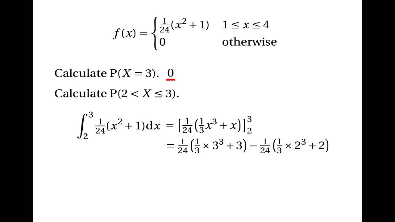
Continuous Random Variables: Probability Density Functions
Probability density functions | Probability and Statistics | Khan Academy

Elementary Statistics - Chapter 5 Probability Distributions Part 1
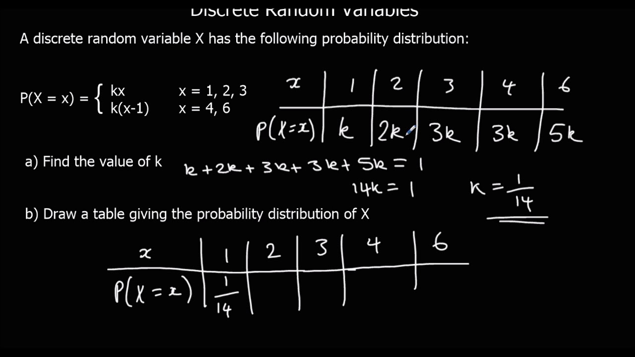
Discrete Random Variables
Constructing a probability distribution for random variable | Khan Academy
5.0 / 5 (0 votes)
Thanks for rating: