Elementary Statistics - Chapter 5 Probability Distributions Part 1
TLDRThe video script delves into the concept of random variables, distinguishing between discrete and continuous types, and their applications. It explains probability distributions, emphasizing they must have probabilities between 0 and 1 that sum to 1. The script illustrates how to calculate mean, variance, and standard deviation for discrete variables, using a calculator for practical examples. It also covers expected value calculations, demonstrating through a raffle scenario the process of determining expected gains or losses.
Takeaways
- 📊 A random variable 'X' is a quantity variable whose values are the result of a random process, such as the number of sales calls made in a day.
- 🔢 There are two types of random variables: discrete, with a finite or countable number of outcomes, and continuous, with an uncountable number of outcomes represented by an interval.
- 📝 Discrete random variables can be listed and include examples like the number of sales calls or mistakes per page, while continuous variables include measurements like length, depth, or time.
- ✅ A probability distribution for a discrete random variable lists each possible value with its corresponding probability, which must be between 0 and 1 and sum up to 1.
- 📈 Probability distributions can be represented in tables, graphs, or mathematical formulas, and they describe the population rather than a sample.
- 🔍 To determine if a table represents a valid probability distribution, check that all probabilities are between 0 and 1 and that they sum to 1.
- 📚 The mean, standard deviation, and variance of a probability distribution are parameters derived from the distribution and are not based on sample statistics.
- 🧮 The mean of a discrete probability distribution is calculated by summing the product of each value and its probability, while variance and standard deviation are calculated using similar summation methods.
- 🔢 For calculating the mean, standard deviation, and variance, rounding rules apply, typically rounding to one more decimal place than the random variable 'X'.
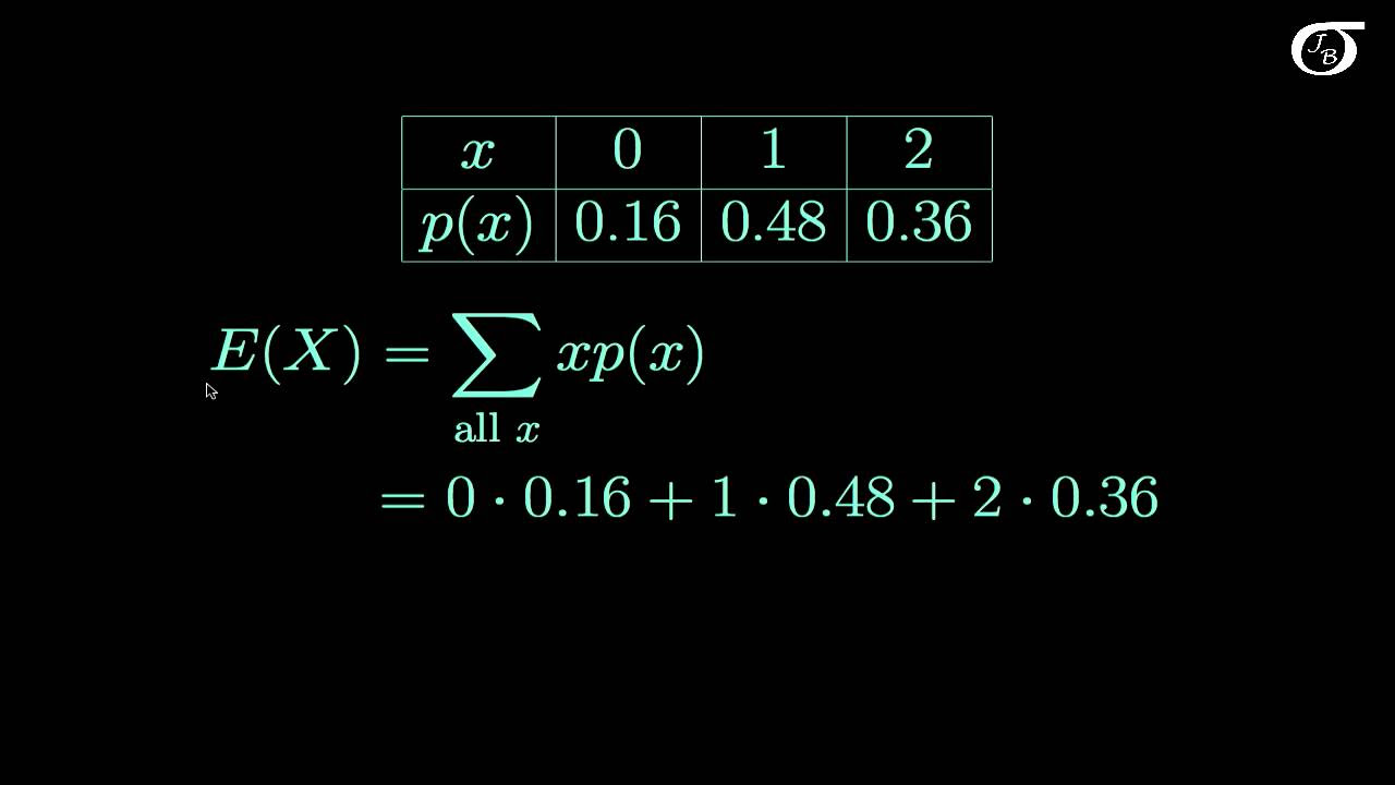
- 🎰 The expected value of a discrete random variable is the same as its mean and is calculated by multiplying each outcome by its probability and summing these products.
- 🏥 An example of applying a probability distribution is calculating the expected number of patients seen in an ER within a given hour, where probabilities are summed for ranges of outcomes.
Q & A
What is a random variable in the context of probability distribution?
-A random variable is a quantity variable whose values are the results of a random process, denoted by the variable X. It can represent various outcomes such as the number of sales calls made in a day or the hours spent on sales calls.
What are the two types of random variables mentioned in the script?
-The two types of random variables are discrete and continuous. Discrete random variables have a finite or countable number of possible outcomes, while continuous random variables have an uncountable number of possible outcomes represented by an interval on the number line.
Can you provide examples of discrete random variables mentioned in the script?
-Examples of discrete random variables include the number of sales calls, the number of calls, shares of stock, and mistakes per page, as they are countable.
What are some examples of continuous random variables?
-Continuous random variables can include length, depth, volume, time, and weight, as they are represented by intervals and are not countable.
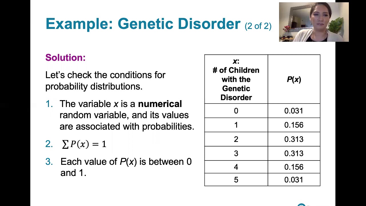
What are the conditions that a probability distribution must satisfy?
-A probability distribution must satisfy two conditions: each probability must be between 0 and 1, and the sum of all probabilities must equal 1.
Can a table with probabilities summing to more than 1 be considered a probability distribution?
-No, a table with probabilities summing to more than 1 does not meet the conditions of a probability distribution, as the sum of probabilities must equal exactly 1.
How can the mean of a discrete probability distribution be calculated?
-The mean of a discrete probability distribution is calculated by summing the product of each possible value of the random variable and its corresponding probability.
What is the expected value of a discrete random variable and how is it calculated?
-The expected value of a discrete random variable, denoted by E(X), is equal to the mean of the random variable. It is calculated by summing the random variable times its probability for each outcome.
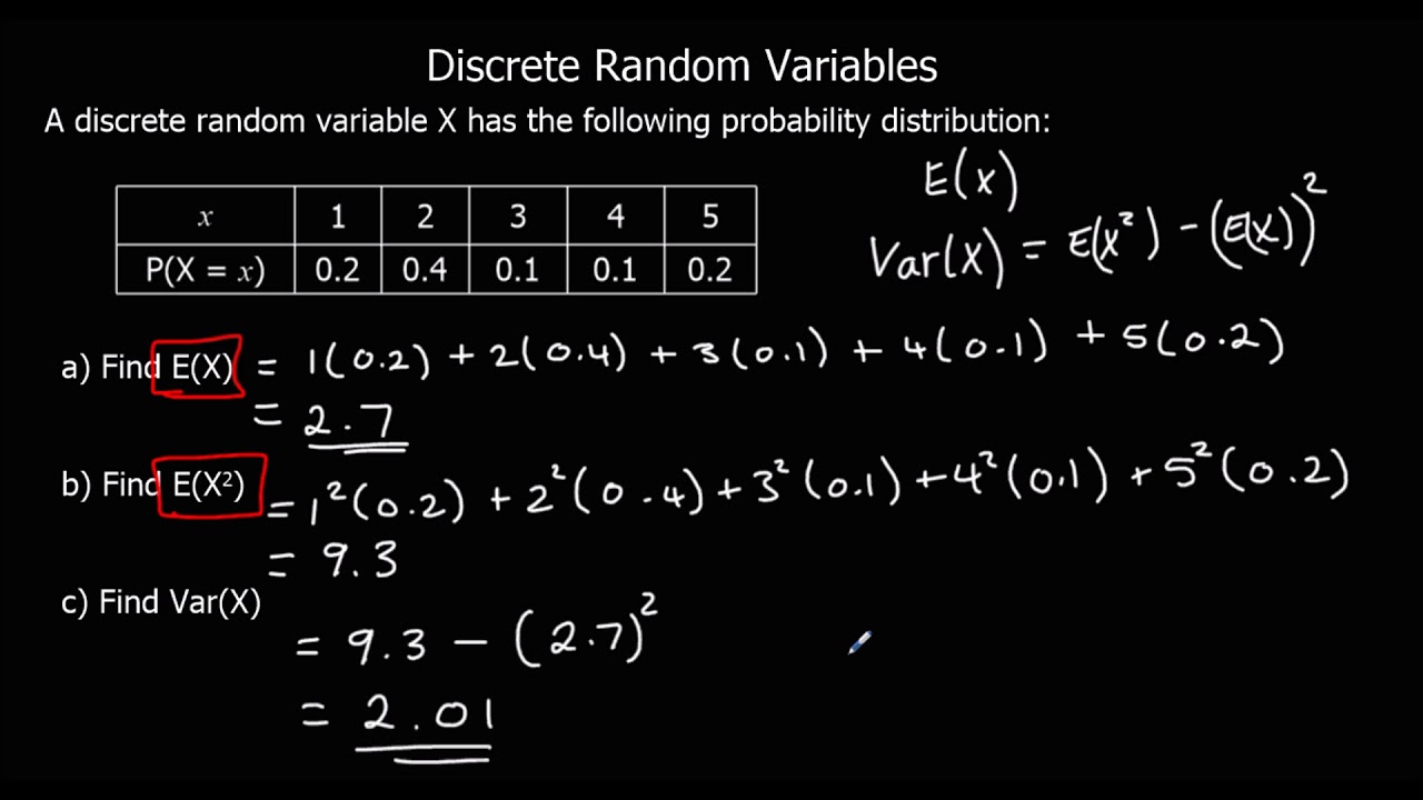
How can the variance and standard deviation of a discrete probability distribution be found?
-The variance is found by summing the square of the difference between each outcome and the mean, multiplied by its probability. The standard deviation is the square root of the variance.
What is the purpose of the rounding off rules for the mean, standard deviation, and variance?
-The rounding off rules ensure consistency in the presentation of results by rounding the mean, standard deviation, and variance to one more decimal place than the number of decimal places used for the random variable X.
Can you explain the concept of expected value using the raffle ticket example from the script?
-The expected value in the raffle ticket example represents the average gain or loss per ticket purchased, taking into account the probabilities of winning each prize and the cost of the ticket. It incorporates both the potential winnings and the cost of participation.
Outlines
📊 Understanding Random Variables and Probability Distributions
This paragraph introduces the concept of random variables as quantities whose values are determined by random processes, denoted by 'X'. It distinguishes between discrete and continuous random variables, with the former having a finite or countable number of outcomes and the latter having an uncountable number represented by intervals. Examples of discrete variables include the number of sales calls or shares of stock, while continuous variables could be time, weight, or volume. The paragraph also explains the conditions for a valid probability distribution, which must have probabilities between 0 and 1 that sum to 1, and can be represented in various forms such as tables, graphs, or mathematical formulas. It provides an example of a table that incorrectly represents a probability distribution due to the sum of probabilities exceeding 1.
📘 Calculating Probabilities and Describing Probability Distributions
The second paragraph delves into calculating specific probabilities from a given distribution, such as the exact number of patients in an ER within an hour. It explains how to interpret probability distributions to answer questions about 'at least' or 'at most' a certain number of outcomes, by summing the relevant probabilities. The paragraph also discusses the parameters of a probability distribution, including mean, standard deviation, and variance, which are considered parameters rather than statistics. It provides formulas for calculating these parameters and emphasizes the importance of rounding off results according to the number of decimal places used for the random variable 'X'. An example using a TI-83 or 84 calculator to find the mean, variance, and standard deviation is given, with step-by-step instructions for data entry and calculation.
🎰 Expected Value and Its Calculation in Discrete Random Variables
This paragraph focuses on the expected value of a discrete random variable, which is denoted by 'E(X)' and is equal to the mean of the variable. It describes how to calculate the expected value by summing the product of each outcome and its corresponding probability. An example of a raffle is used to illustrate the concept, where the expected gain is calculated by considering the cost of the ticket and the probabilities of winning different prizes or losing. The paragraph highlights the importance of including the cost of participation and the possibility of losing when calculating the expected value, and it shows how to construct a probability distribution table to find the expected outcome.
🧮 Applying Probability Distributions to Real-World Scenarios
The final paragraph discusses the application of probability distributions to real-world scenarios, such as the raffle example provided. It explains how to calculate the expected value of a game by considering the actual winnings after ticket costs and the chances of winning versus losing. The paragraph demonstrates the process of determining the probabilities of winning each prize and losing, and then using these probabilities to calculate the overall expected value. It concludes with the insight that, in the given raffle scenario, the expected value indicates a loss for each ticket purchased, providing a practical application of probability distribution concepts.
Mindmap
Keywords
💡Random Variable
💡Discrete Random Variable
💡Continuous Random Variable
💡Probability Distribution
💡Mean
💡Variance
💡Standard Deviation
💡Expected Value
💡Parameters
💡Rounding Rules
Highlights
Random variables are quantities whose values result from random processes, denoted by variable X.
Discrete random variables have a finite or countable number of possible outcomes.
Continuous random variables have an uncountable number of outcomes represented by intervals on a number line.
Examples of discrete random variables include number of sales calls, calls per share, and people in line.
Examples of continuous random variables include length, depth, volume, time, and weight.
A probability distribution lists each possible value of a random variable with its corresponding probability.
Probabilities in a distribution must be between 0 and 1 and the sum of probabilities must equal 1.
Probability distributions can be represented as tables, graphs, or mathematical formulas.
A table of job applicant mistakes during interviews is not a valid probability distribution due to probabilities summing to more than 1.
Probability distributions describe a population, with mean, standard deviation, and variance as parameters, not statistics.
The mean of a discrete probability distribution is calculated as the summation of the random variable times its probability.
Variance and standard deviation of a probability distribution are calculated using summation formulas.
Rounding rules for mean, standard deviation, and variance involve carrying one more decimal place than the random variable X.
To find the mean, variance, and standard deviation for a discrete random variable, use a calculator like the TI-83 or 84.
Expected value of a discrete random variable is denoted by E(X) and is equal to the mean.
In a raffle example, the expected value calculation incorporates actual winnings and the cost of the ticket.
The expected value calculation for the raffle ticket example shows a loss of $1.35 per ticket purchased.
Transcripts
Browse More Related Video
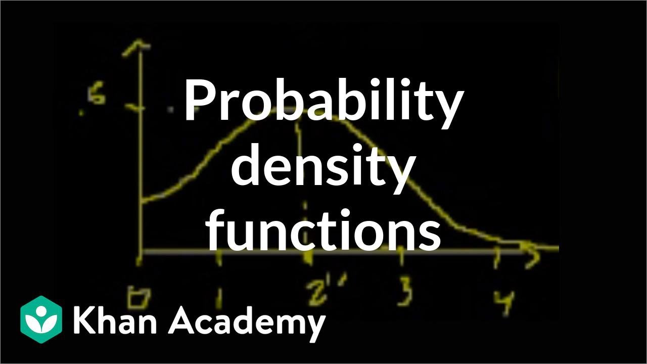
Probability density functions | Probability and Statistics | Khan Academy
5.1.2 Discrete Probability Distributions - Probability Distributions and Probability Histograms
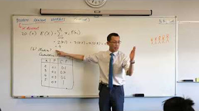
Discrete Random Variables (1 of 3: Expected value & median)
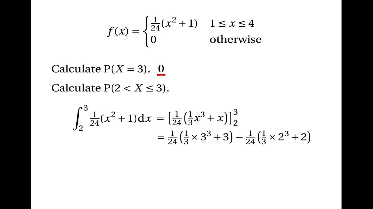
Continuous Random Variables: Probability Density Functions
Expected Value and Variance of Discrete Random Variables
Discrete Random Variables The Expected Value of X and VarX
5.0 / 5 (0 votes)
Thanks for rating: