Continuous Random Variables: Probability Density Functions
TLDRThis video script delves into the concept of probability density functions for continuous random variables, contrasting them with discrete variables like binomial and Poisson distributions. It illustrates how probability density functions, akin to histograms, represent the likelihood of different outcomes, such as alien heights or marathon times. The script explains how to calculate probabilities by integrating under the curve, emphasizing that the function must be non-negative and the total area under the curve equals one. It guides viewers through examples of recognizing valid functions, calculating probabilities, and defining piecewise functions, highlighting the theoretical nature of continuous random variables and their applications.
Takeaways
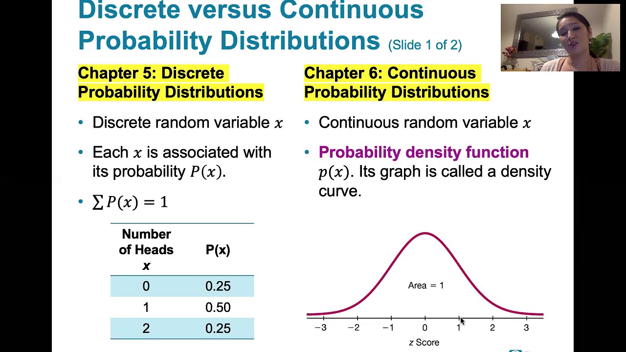
- 📚 A continuous random variable represents outcomes that can take on any value within a range, such as distance or time.
- 📊 Continuous random variables contrast with discrete random variables, which are whole numbers representing counts or occurrences.
- 👽 The probability density function (PDF) illustrates the distribution and relative likelihood of outcomes, using an example of alien heights.
- 📈 The PDF is similar to a histogram, showing the shape of the distribution, but provides a smoother, more detailed picture as intervals increase.
- 🌟 The area under the PDF curve between two points represents the probability of the random variable falling within that range.
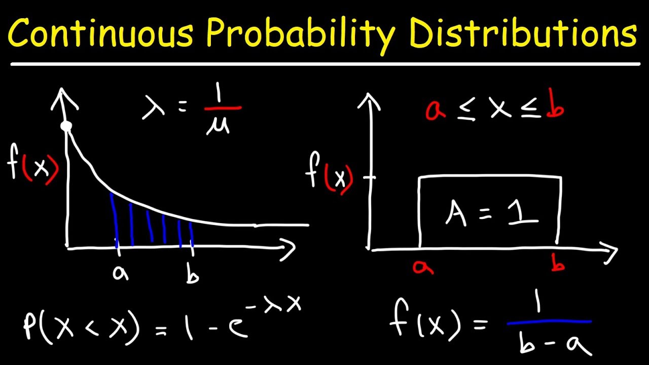
- ∫ To find probabilities, one must integrate the PDF within the desired limits, which may require calculus.
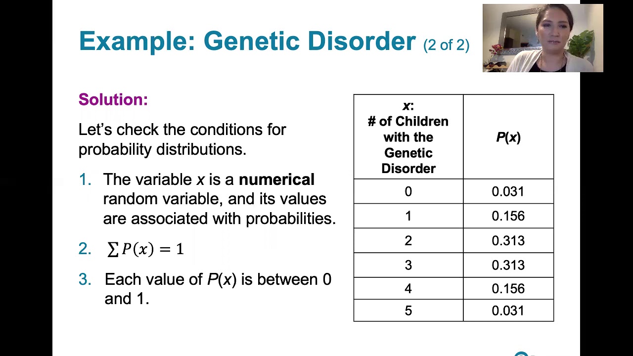
- 🚫 A PDF must never be negative, ensuring all probabilities are non-negative and valid.
- 🔍 The total area under the PDF curve must equal one, reflecting that the sum of all probabilities must equal certainty.
- 🤔 Real-world PDFs can be complex, and theoretical understanding is often more practical than direct calculation.
- 📉 Recognizing valid PDFs involves checking that the function does not dip below the x-axis and that the total area under the curve is one.
- 🧐 Calculating probabilities with PDFs often involves integration, and sometimes simple geometry can be used to find areas under the curve.
Q & A
What is a continuous random variable?
-A continuous random variable is a variable that can take any value within a range, such as the length of a pencil or the finishing time of a marathon runner. It is characterized by measurements of distance or time, which are continuous rather than discrete.
How do continuous random variables differ from discrete random variables?
-Continuous random variables can take any value within a range and are often measurements of distance or time. Discrete random variables, on the other hand, represent counts or whole numbers, such as the number of successes in a sequence of trials or the number of events in a time interval.
What is a probability density function (PDF)?
-A probability density function is a function that describes the likelihood of a continuous random variable taking on a particular value. It provides a sense of the different possible outcomes and their relative probabilities.
How is a probability density function similar to a histogram?
-A probability density function is similar to a histogram in that it shows the shape of the distribution of data points, such as heights of aliens in the video example. Both are used to represent the distribution and relative frequencies of data.
Why can't the probability density function be negative?
-The probability density function cannot be negative because it represents probabilities, which are inherently non-negative. A negative value would imply a negative probability, which is not meaningful in the context of probability theory.
What is the total area under the probability density function and why must it equal one?
-The total area under the probability density function represents the sum of all probabilities for all possible outcomes of the random variable. It must equal one because the certainty of all possible outcomes occurring is 100%, or a probability of one.
How can you find the probability that a continuous random variable falls between two values, a and B?
-The probability that a continuous random variable falls between two values, a and B, is found by calculating the area under the probability density function between those two points. This is done by integrating the PDF from a to B.
What is the significance of integrating the probability density function to find probabilities?
-Integrating the probability density function allows you to find the probability of a continuous random variable falling within a certain range. It is a fundamental operation in continuous probability theory, analogous to summing frequencies in discrete distributions.
Why is it impossible to find the probability that a continuous random variable is exactly a certain value?
-The probability that a continuous random variable is exactly a certain value is impossible to find because the variable can take on an infinite number of values within a range. The area under the curve at a single point (representing a specific value) is zero, as it would require an infinitely thin line with no width.
What is a piecewise defined function and why is it commonly used in probability density functions?
-A piecewise defined function is a function that is defined by different expressions over different intervals of its domain. It is commonly used in probability density functions because it allows for the modeling of complex distributions that change behavior over different ranges of the random variable.
How do you determine if a function could be a probability density function by looking at its graph?
-To determine if a function could be a probability density function by looking at its graph, you should check that the function is non-negative over its entire domain (no part of the graph dips below the x-axis) and that the total area under the curve equals one.
What is the process of finding the value of K in a partially defined probability density function?
-The process involves integrating the function over its entire domain and setting the result equal to one, as the total probability must sum to one. By solving for K, you ensure that the function satisfies the properties of a probability density function.
How can you calculate the probability that a continuous random variable falls within a specific range using integration?
-To calculate the probability that a continuous random variable falls within a specific range, you integrate the probability density function over that range. The result of the integration gives the area under the curve, which represents the probability of the variable falling within that range.
What is the relationship between the probability of a continuous random variable being exactly a certain value and the width of that value?
-The probability of a continuous random variable being exactly a certain value is zero because the width of that value (the range of possible values it could take) is effectively zero. The area under the curve at a single point is zero, as it would require an infinitely thin line with no width.
Why is it necessary to integrate a piecewise defined probability density function in parts?
-It is necessary to integrate a piecewise defined probability density function in parts because the function is defined by different expressions over different intervals. Each part of the function must be integrated separately over its respective interval to find the total probability for a specific range.
How do you find the equation of a line in a piecewise defined probability density function?
-To find the equation of a line in a piecewise defined probability density function, you determine the slope (gradient) and y-intercept (C) of the line. The slope can be found by the change in y over the change in x, and the y-intercept is the point where the line crosses the y-axis.
Outlines
📊 Introduction to Continuous Random Variables and Probability Density Functions
This paragraph introduces the concept of continuous random variables, which are measures of distance or time and can take any value within a range. It contrasts these with discrete random variables, such as those following a binomial or Poisson distribution, which count whole number occurrences. The main focus is on probability density functions (PDFs), which are used to represent the likelihood of different outcomes for continuous variables. An analogy is made with alien heights on an imaginary planet to explain how a PDF can show the distribution and relative likelihood of various heights. The paragraph also touches on how PDFs are similar to histograms but provide a smoother, more detailed picture of the distribution by allowing for an infinite number of intervals.
📈 Understanding Probability Density Functions through Integration and Area
The paragraph delves deeper into the workings of probability density functions, explaining how areas under the curve of a PDF correspond to probabilities of certain outcomes. It uses the example of finding the probability of selecting an alien of a certain height range by calculating the area under the PDF for that range. The importance of integration in finding these areas is highlighted, along with the rules that a PDF must adhere to: it cannot be negative, and the total area under the curve must equal one, representing the certainty of all possible outcomes. The paragraph also discusses the theoretical nature of real-world PDFs and the types of questions one might encounter when dealing with them, such as recognizing valid PDFs and calculating probabilities.
🔍 Recognizing and Defining Probability Density Functions
This section focuses on the ability to recognize and define probability density functions. It provides examples of graphs that could or could not represent a PDF, explaining why certain features, such as a function dipping below the x-axis or failing to integrate to one, disqualify a function from being a PDF. The paragraph also presents a problem involving a piecewise-defined function with an unknown constant, K, and demonstrates how to determine its value by ensuring the total area under the curve equals one. This involves integrating the function over a specified range and solving for K, which in this case is found to be 1/24.
📚 Calculating Probabilities with Probability Density Functions
The paragraph discusses how to calculate probabilities using probability density functions. It clarifies a common misconception by explaining that for continuous random variables, the probability of an exact value is zero, as opposed to discrete variables where exact values are possible. The example provided involves calculating the probability that a continuous random variable X falls within a specific range, demonstrating the use of integration to find the area under the PDF for that range. The calculation involves integrating a piecewise-defined function over the specified limits and provides a clear example of how to approach such problems.
📉 Advanced Integration Techniques for Piecewise-defined Probability Density Functions
This final paragraph illustrates the process of calculating probabilities for piecewise-defined probability density functions using integration. It emphasizes the need to split the function into parts and integrate each part separately when the function's definition changes within the range of interest. The example given involves integrating two different expressions over different limits to find the probability that a continuous random variable falls within a specific interval. The paragraph concludes with a reminder of the key points about probability density functions: the probability of a random variable being between two values is found by integrating the PDF over that interval, the PDF must be non-negative, and the total area under the PDF must equal one.
Mindmap
Keywords
💡Continuous Random Variable
💡Discrete Random Variable
💡Probability Density Function (PDF)
💡Histogram
💡Integration
💡Piecewise Defined Function
💡Total Area Under the Curve
💡Non-Negative Probability Density
💡Calculating Probabilities
💡Theoretical Examples
Highlights
Introduction to continuous random variables as measures of distance or time.
Comparison between continuous and discrete random variables, like binomial and Poisson distributions.
Explanation of probability density functions (PDFs) using an alien height example.
Illustration of PDFs with a graph showing two clusters of alien heights.
Comparison of PDFs to histograms and the process of refining a histogram into a PDF.
Understanding that the area under the PDF curve represents probability.
Calculating probabilities by integrating the PDF between specified limits.
Requirement for PDFs to be non-negative to avoid negative probabilities.
The total area under the PDF curve must equal one, representing total probability.
Theoretical approach to continuous random variables and PDFs without real-world examples.
Recognizing valid PDFs by ensuring the graph does not dip below the x-axis.
Ensuring the total area under a PDF graph equals one for validity.
Solving for K in a piecewise-defined PDF function using integration.
Calculating the probability that a continuous random variable falls within a specific range.
Understanding that the probability of a continuous random variable being exactly a certain value is zero.
Using geometry to find the area under a PDF curve without integration.
Defining a PDF algebraically from a given graph by determining the equations of its parts.
Integrating a piecewise-defined function in parts to find the probability of an event.
Emphasizing the need to integrate piecewise functions with different limits for different parts.
Transcripts
Browse More Related Video
6.1.1 The Standard Normal Distribution - Discrete and Continuous Probability Distributions
Probability density functions | Probability and Statistics | Khan Academy

Session 40 - Probability Distribution Functions - PDF, PMF & CDF | DSMP 2023
Continuous Probability Distributions - Basic Introduction
5.1.2 Discrete Probability Distributions - Probability Distributions and Probability Histograms

Elementary Stats Lesson #11
5.0 / 5 (0 votes)
Thanks for rating: