AP Calculus AB/BC Unit 7 Practice Test
TLDRVin delves into an AP Calculus AB/BC practice test, focusing on Unit 7, which covers differential equations and slope fields. He methodically explains how to solve various problems, from matching slope fields to differential equations to calculating limits and finding particular solutions. Vin provides detailed walkthroughs for each question, employing techniques like process of elimination, chain rule, Euler's method, and logistic differential equations. He emphasizes understanding the underpinnings of each concept, making the session an invaluable resource for students preparing for the AP Calculus exam.
Takeaways
- 📚 Start with understanding the slope field: Positive slope means the curve is increasing, negative slope means it's decreasing, undefined slope indicates a vertical line, and zero slope indicates a horizontal line.
- 🔍 Identify key features in slope fields: Look for zero slopes or vertical slopes as they can help match the field to a differential equation.
- 🧮 Plug in given points to answer choices: This can quickly eliminate incorrect solutions in differential equation problems.
- 📈 Verify solutions by taking derivatives: Ensure that the derivative of the proposed solution fits the original differential equation.
- 🔑 Use the second derivative for concavity: The sign of the second derivative can tell you whether a graph is concave up or down, which helps in approximations.
- 🧷 Find horizontal asymptotes: Setting the derivative equal to zero can help find horizontal asymptotes, which are key features of the solution curve.
- 🔍 Look for direct proportionality: In problems involving rates of change, look for phrases like 'directly proportional' which suggest a relationship of the form y = kx.
- 📉 Sketch solution curves: Use the direction field to sketch the solution curve, ensuring it follows the direction of the slope field and approaches any asymptotes.
- 📐 Use Euler's method for approximations: When no slope field is given, Euler's method can be used to approximate solutions by taking small steps and using the differential equation.
- 📈 Logistic growth has a maximum rate: The fastest growth rate for a logistic function is at the point of inflection, halfway between the initial value and the carrying capacity.
- ➗ Separation of variables is a common technique: It's used to solve differential equations, particularly those that can be written in the form of dy/dx = f(y)g(x).
- 🔠 Partial fraction decomposition is a useful algebraic tool: It helps in integrating complicated rational functions by breaking them into simpler parts.
Q & A
What is the concept of 'slope guy' mentioned in the script?
-The 'slope guy' is a conceptual tool used to visualize the slope of a curve at different points. It helps to identify where the curve is increasing (positive slope), decreasing (negative slope), vertical (undefined slope), or horizontal (zero slope).
How does one determine the differential equation that matches a given slope field?
-To determine the matching differential equation, one should look for features in the slope field such as zero slopes or vertical slopes, and then find an equation in the answer key that has factors leading to the same roots as indicated by these features.
What is the process of verifying a particular solution to a differential equation?
-Verification involves substituting the proposed solution and its derivative into the differential equation to check if the equation holds true. If the left side (the derivative represented by the differential equation) equals the right side after substitution, the proposed function is a solution.
How does one find the limit of a function as x approaches infinity for a given differential equation?
-The limit can be found by analyzing the behavior of the solution curve as x increases without bound. This often involves identifying horizontal asymptotes and the direction of the slope field. The limit is the y-value that the solution curve approaches as x tends to infinity.
What is Euler's method, and how is it used to approximate values in differential equations?
-Euler's method is a numerical technique used to approximate solutions to differential equations. It involves using the derivative of the function at a point to estimate the value of the function at a nearby point. This is done iteratively, taking small steps (using the differential equation) to build an approximation of the function's behavior.
How does the logistic differential equation model population growth?
-The logistic differential equation models population growth by incorporating a carrying capacity, which is the maximum population size that the environment can sustain. The growth rate is fastest at half the carrying capacity and slows as the population approaches the carrying capacity, preventing unlimited exponential growth.
What is the significance of the point of inflection in a logistic growth curve?
-The point of inflection in a logistic growth curve is where the curve changes concavity, from concave up (growth is accelerating) to concave down (growth is decelerating). It represents the point at which the growth rate is at its maximum.
How can one determine if an approximation using a tangent line is an overestimate or an underestimate?
-The determination of whether an approximation is an overestimate or an underestimate depends on the concavity of the curve. If the curve is concave up, the tangent line will lie below the curve, leading to an underestimate. Conversely, if the curve is concave down, the tangent line will lie above the curve, leading to an overestimate.
What is the role of the second derivative in determining the concavity of a function?
-The second derivative of a function indicates the rate of change of the first derivative. If the second derivative is positive, the function is concave up, and if it is negative, the function is concave down. This helps in understanding the overall shape of the function and the behavior of its tangent lines.
How does one solve a differential equation using separation of variables?
-Separation of variables involves rewriting the differential equation so that all terms involving one variable are on one side and the other variable on the opposite side. This often leads to an equation that can be integrated on both sides to find the general solution to the differential equation.
What is the purpose of the initial condition in a differential equation?
-The initial condition provides a specific value for the solution at a given point. It is crucial for determining a particular solution from the general solution of a differential equation, acting as a constraint that allows the calculation of constants within the general solution.
Outlines
📚 Introduction to AP Calculus Practice Test
Vin introduces an AP Calculus practice test, focusing on Unit 7. He mentions providing a link to the test in the video description and outlines his approach to solving differential equations by visualizing a 'slope guy' to match slope fields to their equations. He emphasizes identifying key features like zero slope and vertical lines to find corresponding differential equations.
🔍 Matching Slope Field to Differential Equation
The video script explains how to match a given slope field to its differential equation by looking for specific slope characteristics. It details the process of elimination using the answer choices and verifying them against the slope field, ultimately identifying Choice A as the correct answer.
🧮 Solving Differential Equations with Initial Conditions
Vin demonstrates how to solve for a function given a differential equation and a point on the solution curve. He suggests plugging the point into the answer choices and verifying by taking derivatives. Through this method, he eliminates incorrect options and confirms Choice C as the correct solution.
📐 Analyzing Roman Numeral Equations
The script covers a Roman numeral question where the task is to find an equation that satisfies a given differential equation. Vin uses a brute force approach by finding the second derivative of each Roman numeral option, leading to the conclusion that Roman numeral one is correct.
📈 Finding Expressions for G of T
The video discusses assuming y equals g of T as a solution to a differential equation, with given values for G of T. It explains using exponential models for differential equations and how to identify the correct form of the solution among the answer choices, concluding that Choice D matches the required form.
🤔 Identifying Potential Solution Curves from Slope Fields
Vin talks about finding potential solution curves from slope fields by drawing curves in the direction indicated by the slope field. He uses the concept of asymptotes and basic curves to match the slope field to a solution curve, identifying Choice A as the best option.
🏞️ Sketching Solution Curves with Horizontal Asymptotes
The script explains how to sketch solution curves for a differential equation with a given initial condition. It details finding horizontal asymptotes from the differential equation and using them to sketch the solution curve, concluding that the limit as X approaches Infinity is given by Choice C.
📉 Determining Horizontal Asymptotes and Solution Curves
Vin discusses finding horizontal asymptotes by setting the derivative equal to zero and using this information to sketch the solution curve. He explains that the curve should either increase or decrease between the asymptotes and shows how to find the limit as X approaches Infinity, which matches Choice A.
🐻 Brown Bears Logistic Differential Equation
The script covers a logistic differential equation where the number of brown bears is given by B of T. It explains finding the carrying capacity of the logistic equation and determining the limit as T goes to Infinity, which is the carrying capacity of 100 brown bears.
📝 Sketching Logistic Curves and Growth Rates
Vin explains the concept of logistic curves, their shape, and how they relate to carrying capacity. He discusses finding the point of inflection where the growth rate is the fastest and how to calculate the rate of growth at that point, resulting in five students per minute getting the disease.
🔢 Euler's Method for Approximating Infections Over Time
The script outlines using Euler's method to approximate the number of students infected at a certain time interval. It involves creating a table with time, number of infections, and the derivative, then using the tangent line to approximate values at subsequent time points, resulting in 28 students infected at T equals four minutes.
🧬 Solving the Logistic Differential Equation for a Disease Spread
Vin shows how to solve a logistic differential equation related to a disease spread with an initial condition. He uses partial fraction decomposition and integration to find the particular solution for the number of students infected over time, represented by P of T.
Mindmap
Keywords
💡Slope Field
💡Differential Equation
💡Separation of Variables
💡Logistic Differential Equation
💡Euler's Method
💡Horizontal Asymptote
💡Initial Condition
💡Carrying Capacity
💡Partial Fraction Decomposition
💡Tangent Line Approximation
💡Product Rule
Highlights
The concept of 'slope guy' is introduced to visualize and interpret slope fields in differential equations.
A method for matching slope fields to differential equations by looking for specific characteristics like zero or vertical slopes is presented.
The importance of checking initial conditions when solving for functions in differential equations is emphasized.
A strategy for verifying solutions to differential equations by plugging in points and taking derivatives is demonstrated.
The process of finding the second derivative to validate solutions for differential equations is explained.
An approach to determine the limit of a function as x approaches infinity by analyzing the behavior of the slope field is shown.
The use of Euler's method with a step-by-step guide for approximating values of functions is detailed.
An explanation of how to apply logistic differential equations to model population growth, with an example of brown bears, is provided.
The concept of carrying capacity in logistic growth models and its implications on population limits is discussed.
A technique for sketching solution curves using direction fields and initial conditions for differential equations is demonstrated.
The process of approximating function values using the equation of a tangent line at a given point is explained.
An analysis of whether an approximation is an overestimate or underestimate based on the concavity of the curve is presented.
A comprehensive guide to solving differential equations using separation of variables and integrating is provided.
An example of using Euler's method to approximate the spread of a disease, 'calculitis', among students is given.
An explanation of how to determine the rate of growth when a disease is spreading at its fastest rate using logistic curves is shown.
A step-by-step solution for a logistic differential equation using partial fraction decomposition and integration is demonstrated.
The final solution for the spread of 'calculitis' using logistic differential equations is presented, including the interpretation of the results.
Transcripts
Browse More Related Video
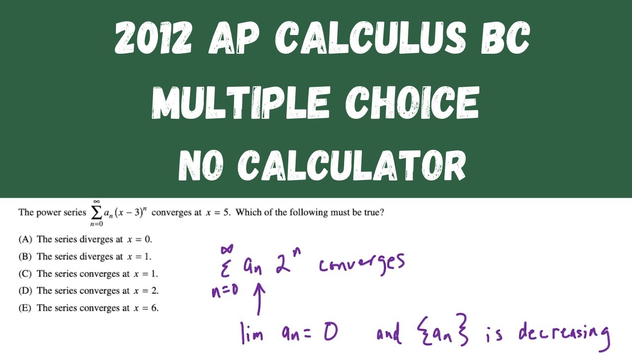
AP Calculus BC Practice Exam 2012 - Multiple Choice questions 1-28
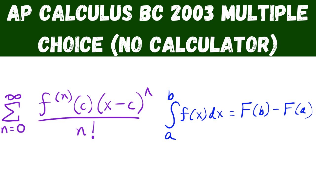
AP Calculus BC 2003 Multiple Choice (no calculator) - questions 1 - 28
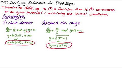
AP Calculus Differential Equations Review (All of Unit 7)
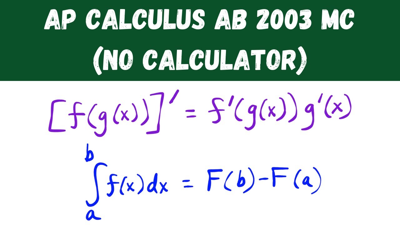
AP Calculus AB 2003 Multiple Choice (no calculator) - Questions 1-28
AP Calc AB & BC Practice MC Review Problems #6

2022 Live Review 2 | AP Calculus BC | Euler's Method, Logistics, and Differential Equations
5.0 / 5 (0 votes)
Thanks for rating: