But what is the Central Limit Theorem?
TLDRThe central limit theorem, a fundamental concept in probability theory, states that the distribution of the sum (or average) of a large number of independent, identically distributed random variables will tend to a normal distribution, regardless of the original distribution. This video script explores the theorem with examples like rolling dice and the Galton board, explaining how the mean and standard deviation change with the sum, and how the normal distribution function is derived. It also discusses the theorem's assumptions and its practical applications, offering a deeper understanding of the underlying mathematical principles.
Takeaways
- 📊 The Galton board demonstrates how chaotic and random single events can still result in predictable relative proportions and distributions, specifically illustrating the normal distribution.
- 📈 The normal distribution, also known as the bell curve or Gaussian distribution, is a prominent statistical distribution that appears in various unrelated contexts, such as demographics and natural numbers.
- 🔑 The central limit theorem is a fundamental concept in probability theory that explains the ubiquity of the normal distribution, stating that the distribution of the sum of a large number of independent, identically distributed random variables increasingly resembles a normal distribution.
- 🎲 The theorem's applicability extends beyond fair dice; it can also be applied to weighted dice, showing that the resulting distribution of sums will still tend toward a bell curve regardless of the initial distribution's skew.
- 🔄 The process of the central limit theorem involves adding multiple samples of a random variable, with the distribution of this sum becoming more bell curve-like as the number of additions increases.
- 🌟 The mean of the distribution increases proportionally with the size of the sum, while the standard deviation increases as the square root of the size of the sum, affecting the spread of the distribution.
- 📐 The standard normal distribution is a special case where the mean is 0 and the standard deviation is 1, playing a crucial role in statistical analysis and allowing for the rescaling of other normal distributions.
- 🤔 The central limit theorem has three underlying assumptions: the variables being added are independent, identically distributed, have a finite variance, and come from the same distribution.
- 📝 The theorem can be formally stated by considering the probability that the standardized sum of variables falls between two real numbers and taking the limit of this probability as the size of the sum approaches infinity.
- 💡 The central limit theorem provides a practical tool for making predictions and estimations, such as determining a range of values within which a sum of random variables is likely to fall with a certain confidence level.
- 🚧 It's important to note that while the central limit theorem is powerful, it does not apply to all situations, particularly when the assumptions of independence, identical distribution, or finite variance are not met.
Q & A
What is the main concept illustrated by a Galton board?
-A Galton board demonstrates how the relative proportions for different outcomes are distributed, particularly showing the emergence of the normal distribution, also known as the bell curve or Gaussian distribution, from a series of random and chaotic events.
What is the significance of the normal distribution in probability theory?
-The normal distribution is significant because it is a common pattern that emerges in many seemingly unrelated contexts, such as the heights of people in a demographic group or the number of distinct prime factors in large natural numbers. It is a fundamental concept in probability theory and statistics.
What is the central limit theorem in probability theory?
-The central limit theorem is a key fact in probability theory that explains why the normal distribution is as common as it is. It states that as the size of the sum of a set of independent, identically distributed random variables increases, the distribution of the sum becomes more like a normal distribution, regardless of the original distribution of the variables.
What are the three assumptions of the central limit theorem?
-The three assumptions of the central limit theorem are: (1) the variables being added are independent of each other, (2) the variables are identically distributed, meaning they all come from the same probability distribution, and (3) the variance of the individual variables is finite.
How does the mean and standard deviation of the sum of random variables change according to the central limit theorem?
-According to the central limit theorem, the mean of the sum of random variables is the sum of their means, and the standard deviation of the sum is the square root of the sum of their variances. As the number of variables increases, the mean increases linearly with the size of the sum, and the standard deviation increases proportionally to the square root of the size of the sum.
What is the empirical rule of thumb related to normal distributions?
-The empirical rule of thumb related to normal distributions states that approximately 68% of the values fall within one standard deviation of the mean, 95% within two standard deviations, and 99.7% within three standard deviations of the mean.
How can the central limit theorem be used to make predictions about a large number of events?
-The central limit theorem can be used to make predictions by allowing us to estimate the range within which a certain percentage of outcomes are likely to fall. For example, if we know the mean and standard deviation of a distribution, we can predict that 95% of the outcomes will be within two standard deviations of the mean, which can be calculated using the theorem's principles.
What happens to the distribution of sums when the number of random variables being added increases?
-As the number of random variables being added increases, the distribution of the sums becomes more symmetric and bell curve-like, regardless of the original distribution of the individual variables. This is a direct result of the central limit theorem.
How does the Galton board model illustrate the central limit theorem?
-The Galton board model illustrates the central limit theorem by showing that even when individual outcomes are unpredictable, the overall distribution of many such outcomes follows a predictable pattern (the normal distribution). The model shows that the final position of a ball after multiple bounces tends to follow a bell curve, despite the randomness of each bounce.
What is the role of the number e and pi in the formula for the normal distribution?
-In the formula for the normal distribution, the number e (Euler's number) is used as the base of the exponent to describe exponential growth or decay. The constant pi appears in the formula because it is a result of ensuring that the area under the curve, which represents the total probability, equals 1. The formula is divided by the square root of pi to normalize the area of the curve.
How does the central limit theorem apply to rolling dice?
-The central limit theorem can be applied to rolling dice by considering the sum of many dice rolls. Regardless of the initial distribution of outcomes for a single die roll, as the number of dice rolls increases, the distribution of the sum of the rolls approaches a normal distribution. This allows us to make predictions about the likelihood of obtaining a certain total sum.
Outlines
🎲 Introduction to the Galton Board and Normal Distribution
The video begins with an introduction to the Galton board, a device that demonstrates the normal distribution or bell curve through the random drop of balls onto a set of pegs. The narrator explains how the relative proportions of different outcomes are distributed, highlighting the prevalence of the normal distribution in various unrelated contexts, such as human height or prime factors in natural numbers. The central limit theorem, a key concept in probability theory, is introduced as an explanation for the ubiquity of the normal distribution. The lesson aims to provide a foundational understanding of the central limit theorem and normal distributions, assuming minimal background knowledge. The video also sets up an overly simplified model of the Galton board to illustrate the central limit theorem, emphasizing that the goal is to provide an illustrative example rather than an accurate physical model.
📈 The Central Limit Theorem and Its Implications
This paragraph delves into the central limit theorem, explaining that as the size of a sum of random variables increases, the distribution of that sum increasingly resembles a bell curve. The lesson's objective is to provide a quantitative understanding of this theorem, enabling predictions about the likelihood of outcomes. The video poses a question to the viewer: given 100 rolls of a die, can one determine a range within which the sum of the rolls is likely to fall with high confidence. The theorem's assumptions are mentioned but not revealed, inviting the viewer to observe and predict what they might be. The video also contrasts a fair die with a weighted die, showing that the core idea of the theorem remains valid regardless of the initial distribution. Simulations are run to visually demonstrate how the distribution of sums evolves towards a bell curve as the sample size increases.
🔢 Understanding Random Variables, Mean, and Standard Deviation
The video continues by explaining the concept of random variables, which are numbers associated with outcomes of a random process. The mean and standard deviation of a distribution are introduced as key measures of central tendency and dispersion. The mean is calculated as the expected value of the random variable, while the standard deviation quantifies the spread of the distribution. The video emphasizes the central limit theorem's relevance to the mean and standard deviation, noting that the mean of the sum of random variables is the sum of their means, and the standard deviation of the sum is the square root of the number of variables times the original standard deviation. This section aims to provide a clear understanding of these concepts to support the viewer's comprehension of the central limit theorem.
📊 Distribution of Sums and the Role of Convolution
The video further explores the distribution of sums of random variables, using the concept of convolution to describe the process. Convolution is a mathematical operation that combines two distributions to produce a third, representing the distribution of their sum. The video demonstrates this through the example of rolling dice, where the distribution of the sum can be calculated by multiplying probabilities of individual outcomes and adding them together. The video shows how the resulting distribution changes with the number of dice rolled, and how it increasingly resembles a bell curve. The video also discusses the computation of distributions for non-uniform dice, emphasizing that the central limit theorem holds regardless of the initial distribution's shape. The section aims to illustrate the process of convolution and its role in the central limit theorem.
📈 Quantitative Description of the Central Limit Theorem
This section focuses on providing a quantitative description of the central limit theorem. The video explains how to realign and rescale distributions so that their means align and their standard deviations equal one. It introduces the formula for a normal distribution, explaining the significance of the constants e (Euler's number) and pi, and how they relate to the bell curve's shape. The video also discusses the importance of the area under the curve representing the total probability of an event occurring. The section aims to give the viewer a clear understanding of the normal distribution's mathematical formulation and its connection to the central limit theorem.
🎲 Applying the Central Limit Theorem to Dice Rolls
The video applies the central limit theorem to a practical example: rolling a fair die multiple times and summing the results. It explains how to use the theorem to predict the range within which the sum is likely to fall with a certain level of confidence. The video demonstrates how to calculate the mean and standard deviation for the sum of dice rolls, and how these values can be used to find the desired range. It also discusses the empirical average of the die rolls and how the central limit theorem can be used to determine the expected range for this average. The section aims to show the practical application of the central limit theorem in solving probability problems.
📝 Assumptions and Limitations of the Central Limit Theorem
The video concludes by discussing the assumptions and limitations of the central limit theorem. It outlines the three assumptions: independence of random variables, identical distribution for all variables, and finite variance. The video explains why these assumptions are necessary and provides an example of a situation where they might not hold, using the Galton board. It also cautions against assuming normal distribution without justification and highlights the importance of finite variance. The section aims to provide a comprehensive understanding of the central limit theorem, its applications, and its limitations.
Mindmap
Keywords
💡Galton Board
💡Normal Distribution
💡Central Limit Theorem
💡Random Variable
💡Mean
💡Standard Deviation
💡Exponential Growth/Decay
💡Variance
💡Probability Density Function
💡Empirical Average
💡Independence
Highlights
The Galton board is a demonstration of how chaotic and random events can lead to predictable distributions.
The normal distribution, also known as the bell curve or Gaussian distribution, is a prominent distribution in probability.
The central limit theorem explains the prevalence of the normal distribution in various seemingly unrelated contexts.
The central limit theorem states that the distribution of the sum of a large number of independent, identically distributed random variables approaches a normal distribution.
The mean and standard deviation of a distribution are key in understanding the central limit theorem and its implications.
The standard deviation grows in proportion to the square root of the size of the sum, which is crucial for the central limit theorem.
The normal distribution function is described by an elegant mathematical formula involving e (the base of natural logarithms) and pi.
The central limit theorem applies to any distribution, regardless of its initial shape.
The central limit theorem has three assumptions: independence of variables, identical distribution, and finite variance.
The central limit theorem can be used to make predictions about the likelihood of outcomes in various scenarios, such as rolling dice.
The empirical average of a large sample can be predicted to fall within a certain range with a high degree of confidence due to the central limit theorem.
The central limit theorem allows for the computation of the distribution of sums without needing to know the exact distribution of the individual variables.
The central limit theorem is a fundamental concept in probability theory with wide-ranging applications in statistics and other fields.
Understanding the central limit theorem provides insight into how order can emerge from chaos in certain random processes.
The central limit theorem can be visually demonstrated through simulations, showing the transition from various initial distributions to a normal distribution.
Transcripts
Browse More Related Video

Lecture 5: Law of Large Numbers & Central Limit Theorem

Introduction to the normal distribution | Probability and Statistics | Khan Academy

Convolutions | Why X+Y in probability is a beautiful mess

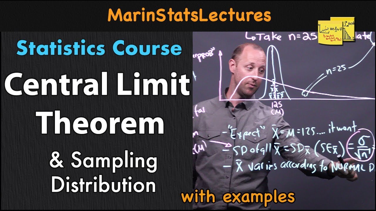
Central Limit Theorem & Sampling Distribution Concepts | Statistics Tutorial | MarinStatsLectures

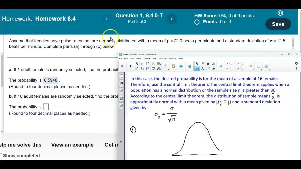
Math 14 HW 6.4.5-T Using the Central Limit Theorem

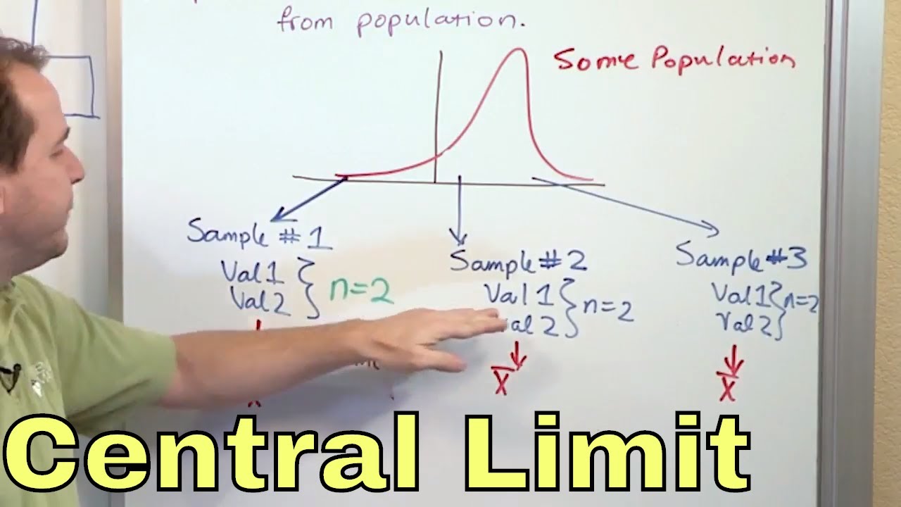
02 - What is the Central Limit Theorem in Statistics? - Part 1
5.0 / 5 (0 votes)
Thanks for rating: