Convolutions | Why X+Y in probability is a beautiful mess
TLDRThe video script delves into the concept of convolution, a fundamental operation in probability that combines two random variables to form a new distribution. It begins with a quiz on the distribution of the sum of two normally distributed random variables and proceeds to explain the concept using the analogy of rolling weighted dice. The script introduces two visualization techniques for convolution: diagonal slices and multiplication tables, and extends these methods to continuous functions and the central limit theorem. The video aims to provide an intuitive understanding of convolution and its role in probability, particularly in understanding the emergence of normal distributions in various probabilistic scenarios.
Takeaways
- 📊 The normal distribution is characterized by its bell curve shape, where the probability of a sample falling within a range is equal to the area under the curve in that range.
- 🎲 The sum of two random variables, each drawn from a normal distribution, behaves like its own random variable, following a distribution that can be determined through convolution.
- 🔍 Convolution is a mathematical operation that combines two probability distributions to produce a third, describing the distribution of their sum. It is denoted with an asterisk (*).
- 🎯 The process of convolution can be visualized in two ways: as diagonal slices in a 3D plot or as the product of two functions along a specific diagonal.
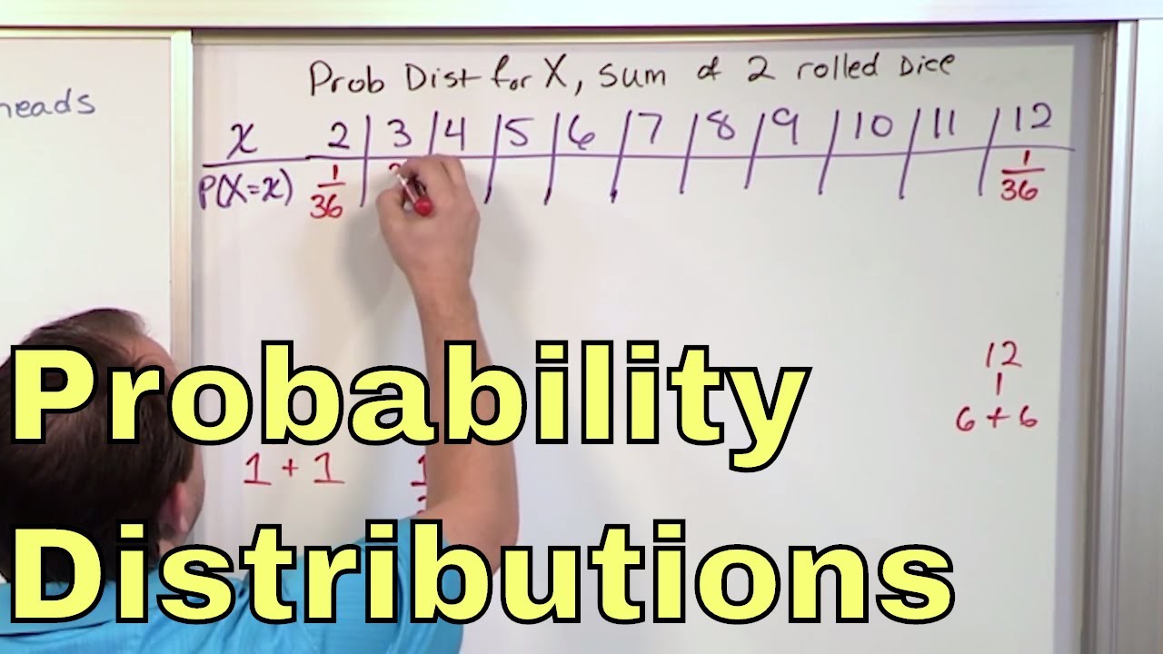
- 🎲 The script uses the example of rolling two weighted dice to illustrate the concept of convolution in a discrete setting, emphasizing the independence of random variables.
- 📈 In the continuous case, the probability density function (PDF) replaces the probability function, and the integral replaces the sum in the convolution formula.
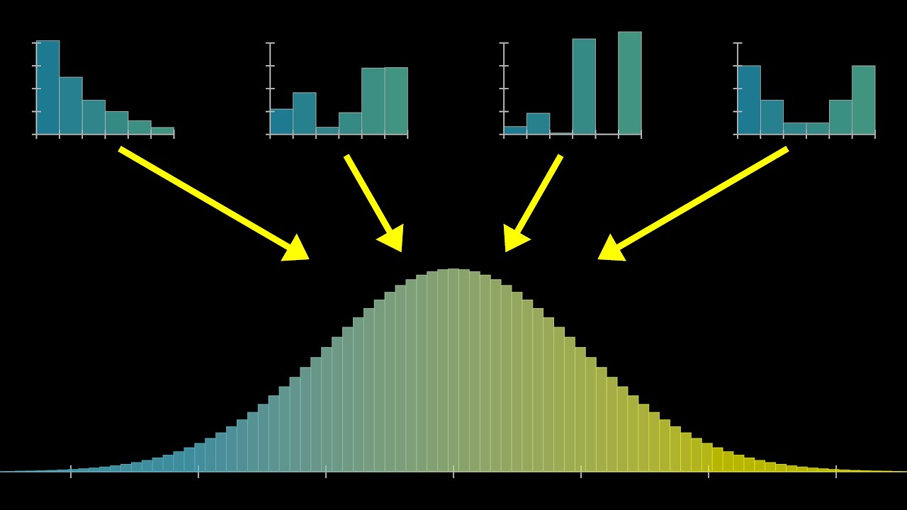
- 🔄 The central limit theorem states that as you repeatedly convolve a distribution with itself, the resulting distribution increasingly resembles a normal distribution, regardless of the original distribution's shape.
- 📊 The convolution operation is symmetric, meaning that the order in which two distributions are convolved does not affect the result.
- 🤔 Understanding convolution is crucial for grasping why normal distributions play a special role in probability and statistics.
- 🚀 The script hints at a more engaging method for calculating the convolution of two normal distributions, which will be explored in the next video.
- 🌟 The visualization of convolution, especially through diagonal slices, not only aids in understanding the concept but also has practical applications in proofs and calculations.
Q & A
What is the main concept being introduced in the script?
-The main concept introduced in the script is the operation of convolution, particularly in the context of combining two random variables to form a new distribution.
How is the distribution of the sum of two random variables related to the original distributions?
-The distribution of the sum of two random variables can be found by convolving the original distributions. This new distribution describes the probabilities of different sums occurring.
What is the role of independence in the context of convolution?
-In the context of convolution, the assumption of independence between the random variables is crucial. It allows the probabilities of outcomes to be multiplied together when computing the combined distribution.
What is the central limit theorem mentioned in the script, and what does it imply?
-The central limit theorem is a fundamental concept in probability that states that as you repeatedly convolve a distribution with itself, the resulting distribution increasingly resembles a normal distribution, regardless of the original distribution's shape.
How does the script illustrate the concept of convolution?
-The script illustrates the concept of convolution through two different visualizations: one using a multiplication table analogy and the other using diagonal slices of a three-dimensional plot. These visualizations help to clarify how the convolution operation combines two distributions to form a new one.
What is the significance of the bell curve shape in the context of the central limit theorem?
-The bell curve shape is significant because it represents the normal distribution, which is the limiting distribution that emerges when applying the central limit theorem. This suggests that the normal distribution is a kind of 'attractor' for sums of random variables.
How does the script relate the concept of convolution to the calculation of probabilities?
-The script relates convolution to the calculation of probabilities by showing how to compute the probability of achieving a specific sum from two random variables. This is done by integrating (or summing, in the discrete case) the product of the individual probability density (or probability mass) functions over all possible pairs of values.
What is the role of the standard deviation in the context of the central limit theorem?
-The standard deviation plays a role in the central limit theorem by determining the spread of the resulting normal distribution after the convolution process. The repeated convolution effectively flattens out the distribution, and rescaling the x-axis ensures that the standard deviation of the resulting distribution is one.
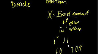
How does the script transition from discrete to continuous distributions?
-The script transitions from discrete to continuous distributions by first introducing the concept of convolution with a simple example of rolling dice, and then moving on to continuous distributions where random variables can take on any real number value. The continuous case involves probability density functions and integrals instead of probabilities and sums.
What is the practical application of understanding convolution in probability?
-Understanding convolution in probability is important for modeling and predicting the outcomes of complex systems where multiple random variables interact. It is fundamental in fields such as statistics, finance, physics, and engineering for analyzing and making predictions based on the combined effects of various random factors.
Outlines
📊 Introduction to Probability Distributions and Quiz
The video begins with a quiz to engage the audience, introducing the concept of normal distribution and random variables. It explains how the shape of the bell curve represents the probability of a sample falling within a specific range of values. The quiz challenges viewers to determine the distribution of the sum of two random variables, one with a normal distribution and the other slightly more spread out. The video sets the stage for a deeper exploration of probability, leading into the concept of convolution and its role in understanding the central limit theorem. It also mentions a previous video on a related topic, emphasizing that this video will focus on continuous functions and provide a more general lesson on adding random variables.
🎲 Visualizing Convolution with Discrete Random Variables
This paragraph delves into the concept of convolution using a discrete example of rolling two weighted dice. It explains how the sum of the rolls follows a new distribution, which can be computed using two visualization methods. The first method involves creating a 6x6 grid to represent all possible outcomes and multiplying probabilities along diagonals to find the probability of specific sums. The second method uses a three-dimensional plot to visualize the probability of different sums, highlighting how the distribution of sums can be seen as collapsing the full distribution along diagonal slices. The paragraph emphasizes the importance of the independence of random variables in these computations.
📈 Formulating Convolution for Discrete Random Variables
The paragraph focuses on the mathematical formulation of convolution for discrete random variables. It introduces the concept of probability density functions and explains how to compute the distribution of the sum of two random variables using a formula that involves summing pairwise products of probabilities. The paragraph also addresses a quirk in the formula where certain values may fall outside the defined domain, explaining that these values are considered to have a probability of zero. It transitions the discussion towards continuous distributions, setting the stage for the next part of the video.
📊 Understanding Continuous Distributions and Convolution
This paragraph shifts the focus to continuous distributions, where random variables can take on any value in an infinite range. It explains the concept of probability density and how it differs from discrete probability. The paragraph introduces the formula for convolution in the continuous case, which involves integrating the product of two probability density functions over all possible values of one variable, while the other variable is adjusted to maintain a constant sum. It also provides an interactive demo to visualize the convolution process, highlighting how the shape of the product graph and the corresponding area change as the sum parameter varies.
📊 Convolution and the Central Limit Theorem
The paragraph explores the central limit theorem, which states that as you take repeated convolutions representing larger and larger sums of a given random variable, the distribution describing that sum approaches a normal distribution, regardless of the original distribution's shape. It discusses why normal distributions are the result of this process and introduces a new visualization method for convolution in the continuous case, which involves creating a three-dimensional graph to represent all possible outcomes and their probability densities. The paragraph explains how integrating along diagonal slices of this graph gives the values of the convolution, providing a deeper understanding of the process.
🎥 Conclusion and Preview of Next Video
The video concludes with a summary of the intricate process of adding two random variables and the beauty of the convolution operation. It acknowledges the complexity of the mathematical formulations while highlighting the value of visual aids in understanding these concepts. The paragraph leaves the audience with a teaser for the next video, where the opening quiz question about adding two normally distributed random variables will be answered using a fun method that leverages the diagonal slice visualization. It encourages viewers to predict what the 3D graph of two normal distributions might look like and how it can be used to understand the central limit theorem.
Mindmap
Keywords
💡Normal Distribution
💡Random Variable
💡Convolution
💡Probability Density Function (PDF)
💡Independent Random Variables
💡Central Limit Theorem
💡Diagonal Slices
💡Continuous Functions
💡3D Plot
💡Sum of Random Variables
Highlights
The concept of a normal distribution and its bell curve shape is introduced, providing a foundation for understanding probability and random variables.
The probability of a sample falling within a specific range of values is explained as the area under the curve in that range, which is a fundamental concept in probability.
A quiz is presented to engage the audience and encourage active thinking about the distribution of the sum of two random variables.
The concept of convolution is introduced as a method for combining two probability distributions to find the distribution of their sum.
The importance of understanding the underlying assumptions, such as independence of random variables, is emphasized for accurate analysis and application.
A practical example of rolling weighted dice is used to illustrate the concept of convolution in a more tangible and relatable manner.
Two distinct visualization methods for convolution are presented: one using a multiplication table grid and the other using a three-dimensional plot, enhancing comprehension through different perspectives.
The concept of probability density and the probability density function (PDF) are explained for continuous random variables, which is crucial for working with real-world applications.
The analogy between discrete and continuous cases is used to bridge the gap in understanding the mathematical operations involved in convolution.
An interactive demo is introduced to help visualize the convolution process for continuous functions, making the abstract concept more accessible and intuitive.
The central limit theorem is mentioned as a key application of convolution, highlighting its importance in probability and statistics.
A detailed explanation of how to compute the distribution of the sum of two random variables using convolution is provided, offering a clear methodology for solving such problems.
The concept of independence of random variables is reiterated as a critical assumption in the analysis and application of convolution.
The process of convolution is described as a smoothing operation that can transform the distribution of the sum of random variables, leading to a better understanding of their behavior.
The potential of using convolution to model real-world phenomena such as weather, finance, and wait times is discussed, showcasing its broad applicability.
The transition from discrete to continuous distributions is explained, with a focus on the mathematical adjustments required for this shift.
The concept of a convolution as combining two functions to produce a new function is introduced, providing a new perspective on this mathematical operation.
The importance of visualizing and understanding the process of convolution is emphasized for a deeper comprehension of probability distributions and their sums.
Transcripts
Browse More Related Video
But what is the Central Limit Theorem?

Session 40 - Probability Distribution Functions - PDF, PMF & CDF | DSMP 2023
Introduction to Random Variables
02 - Random Variables and Discrete Probability Distributions
Introduction to Discrete Random Variables and Discrete Probability Distributions

Elementary Stats Lesson #12
5.0 / 5 (0 votes)
Thanks for rating: