Graphing Higher-Degree Polynomials: The Leading Coefficient Test and Finding Zeros
TLDRIn this educational video, Professor Dave delves into the techniques for graphing higher-degree polynomial functions, beyond the simpler quadratic ones. He introduces viewers to the leading coefficient test, a method that determines a polynomial's end behavior based on its leading term. By examining whether the leading coefficient is positive or negative, and the degree of the polynomial is even or odd, one can predict the function's behavior towards infinity. The video also covers finding the function's zeroes and understanding their multiplicity, which influences how the graph interacts with the x-axis. These foundational concepts enable viewers to sketch approximate graphs of higher-degree polynomials, providing essential insights without delving into the complexities of calculus.
Takeaways
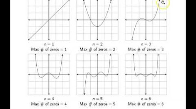
- 😀 Polynomial functions can have complex shapes with hills and valleys, but have predictable end behavior
- 👍 Use the leading coefficient test to determine if a polynomial will rise or fall at the ends
- ✏️ Find x-intercepts (zeroes) to plot key points and understand if the graph will cross or touch the x-axis
- 📐 Factor polynomials or use synthetic division to find the zeroes
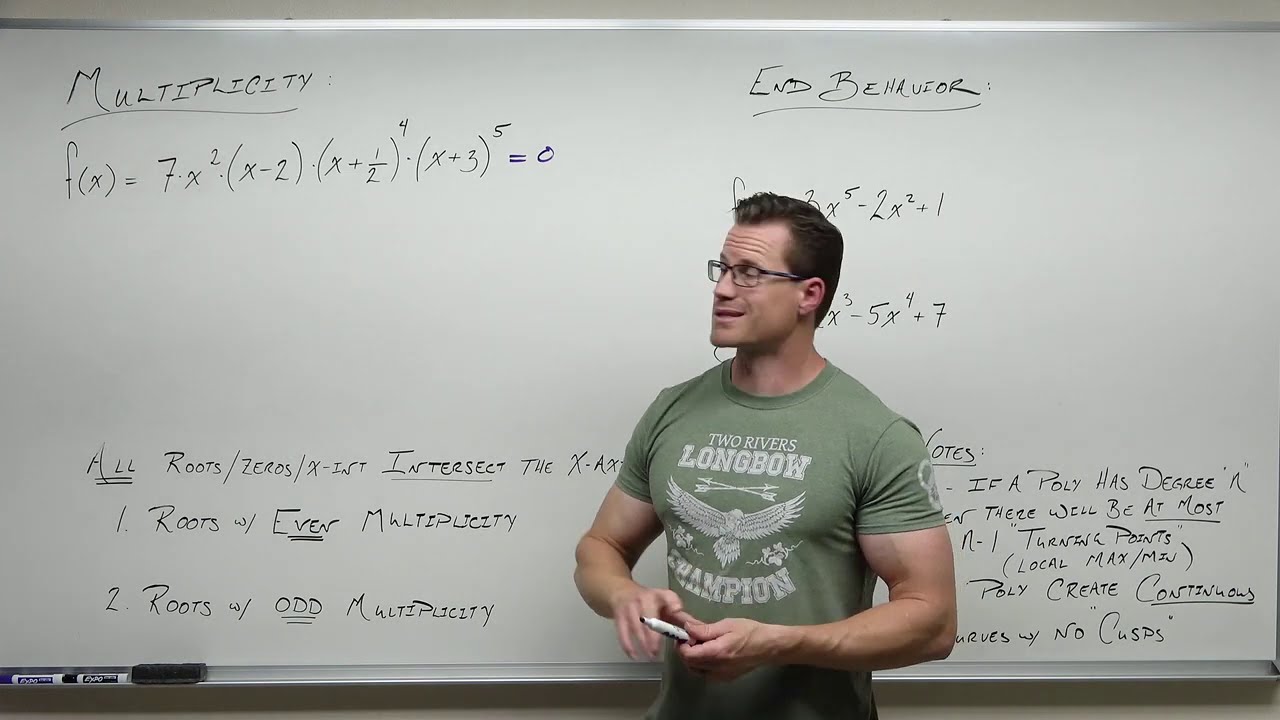
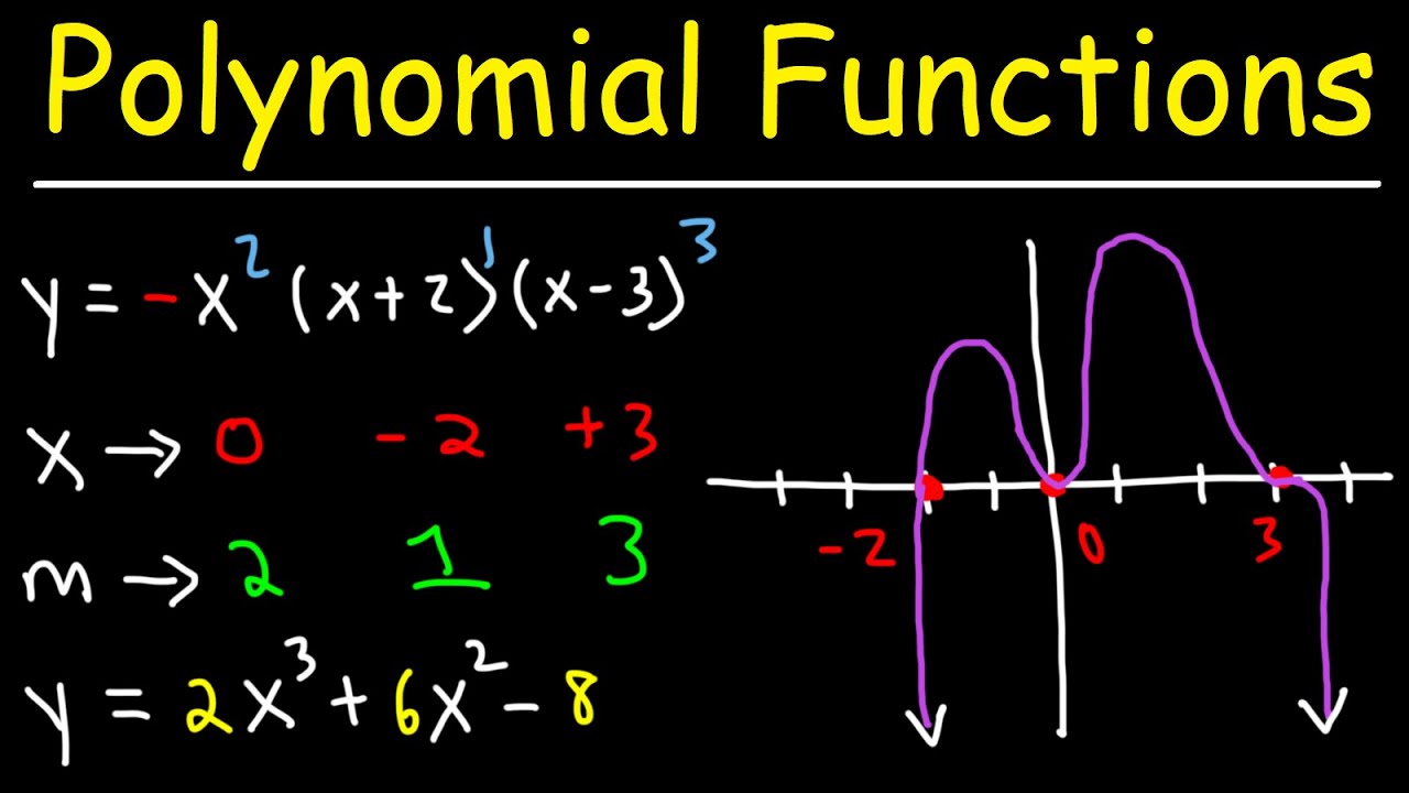
- 🤔 Assess the multiplicity of zeroes - odd means it crosses the x-axis, even means it touches
- 📈 Get the y-intercept by plugging in 0 for x
- 🖋 If a zero has odd multiplicity, the graph crosses the x-axis at that point
- 🖋 If a zero has even multiplicity, the graph touches the x-axis and turns around
- 🎯 Follow the end behavior and plot the key points to sketch the full graph
- 🔁 Watch the video again if you don't understand the concepts
Q & A
What is a leading coefficient test and how is it used to determine end behavior of polynomial functions?
-The leading coefficient test looks at the coefficient and exponent of the leading term (the term with the largest exponent) in a polynomial function. If the exponent is odd and the coefficient is positive, the function falls to the left and rises to the right. If the exponent is odd and the coefficient is negative, the function rises to the left and falls to the right. If the exponent is even and the coefficient is positive, the function rises on both sides. If the exponent is even and the coefficient is negative, the function falls on both sides.
How can you find the x-intercepts or zeros of a polynomial function?
-To find the x-intercepts or zeros, set the polynomial equal to 0 and solve for x. This can be done by factoring the polynomial or using the rational roots test and synthetic division. The values of x that make the function equal 0 are the zeros.
What is the difference between a zero with odd multiplicity versus even multiplicity in terms of graphing?
-If a zero has an odd multiplicity (occurs once or three times etc.), the function will cross the x-axis at that value. If the zero has an even multiplicity (occurs twice or four times etc.), the function will touch the x-axis at that value and curve back in the direction it came from.
Why is finding maxima and minima from a sketch not very precise?
-To accurately find the maxima and minima of a polynomial function requires calculus. The sketching method described provides an approximate graphical shape but does not perfectly identify the precise peaks and valleys.
What are some examples of higher degree polynomial functions?
-Cubic functions (degree 3), quartic functions (degree 4), quintic functions (degree 5), sextic functions (degree 6), and so on. These have terms with exponents larger than 2.
Is it possible to sketch an accurate graph of a high degree polynomial by only finding zeros and end behavior?
-Yes, a reasonably accurate sketch can be obtained from just the end behavior, zeros, and possibly the y-intercept. While not perfectly precise, this provides a good general shape and behavior of the function.
What causes the unpredictable behavior of higher degree polynomial functions compared to lines and parabolas?
-The higher exponents lead to more turns and inflection points in the graph, which is harder to anticipate compared to the consistent shapes of lines and parabolas.
What are some ways to easily get additional points to improve a sketch of a polynomial function?
-The y-intercept can be quickly found by plugging in 0 for x. The zeros can be checked by plugging them into the original function to get associated y values. Maximum/minimum guesses could also be plugged in to get more points on the curve.
What is meant by the continuity and smoothness of polynomial functions?
-Continuous means there are no breaks or discontinuities in the graph - it can be drawn without lifting pencil from paper. Smoothness refers to the lack of sharp corners or cusps - polynomials have rounded peaks and valleys.
What is the benefit of being able to sketch graphs of higher degree polynomial functions?
-It allows for a quick, visual understanding of the general pattern and behavior of the function, without needing to precisely calculate multiple points. The sketch provides an intuitive feel for how the function changes.
Outlines
📈 Graphing Higher-Degree Polynomials
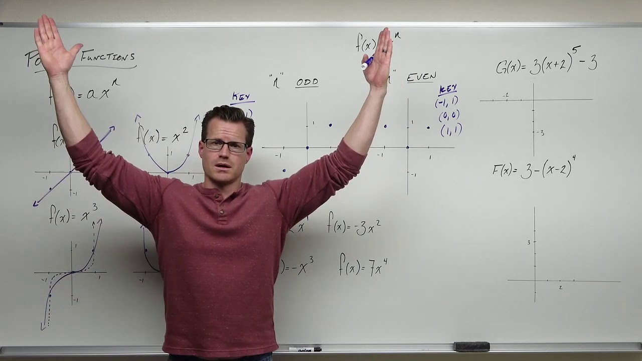
Professor Dave introduces the complexities of graphing higher-degree polynomial functions beyond quadratic ones, like cubic and quartic functions. These functions, being smooth and continuous, exhibit challenging behaviors, including unpredictable hills and valleys. A key technique for sketching these functions involves understanding their end behavior through the leading coefficient test, which determines the function's direction as it extends towards infinity based on the leading term's exponent and coefficient. The process of finding a function's zeroes, or x-intercepts, is also crucial, as these are points where the function equals zero. Factoring and the rational roots test, combined with synthetic division, are methods used to identify these zeroes. The summary underscores the initial steps in graphing higher-degree polynomials by determining their end behavior and zeroes, providing a foundational strategy for sketching their rough outlines.
🔍 Understanding Zeros and Their Multiplicity
This section delves into the significance of the zeroes of a function, specifically how their multiplicity affects the graph of higher-degree polynomials. If a zero appears once, the function crosses the x-axis at that point. However, if a zero is repeated, the function touches the x-axis at that value and then turns back. Professor Dave illustrates this with an example of a quartic function, explaining how zeroes with odd multiplicities (e.g., 1, 3) ensure that the function crosses the x-axis, whereas even multiplicities (e.g., 2) result in the function merely touching the x-axis and turning around. This insight is crucial for graphing polynomials, as it helps predict their shape. Additionally, finding the y-intercept by plugging in zero for x offers another easy point for sketching the graph. This strategy, combined with understanding end behavior and zeroes' multiplicity, equips learners with a solid approach to graphing higher degree polynomials.
Mindmap
Keywords
💡Higher-degree polynomials
💡Leading coefficient test
💡End behavior
💡Zeroes of a function
💡Multiplicity
💡Factoring
💡Rational roots test
💡Synthetic division
💡X-intercepts
💡Y-intercept
Highlights
Introduction to graphing higher-degree polynomials beyond quadratic functions.
Challenges of plotting points and unpredictable behavior of higher-degree functions.
Polynomial functions of degree two or higher are smooth and continuous.
End behavior of polynomial functions depends on the leading term's exponent and coefficient.
The Leading Coefficient Test helps determine the function's end behavior.
Odd exponents with positive coefficients result in functions that fall left and rise right.
Odd exponents with negative coefficients lead to functions rising left and falling right.
Even exponents with positive coefficients make functions rise on both sides.
Even exponents with negative coefficients cause functions to fall on both sides.
Finding zeroes of the function is crucial for sketching its graph.
Zeroes of the function can be found through factoring or the Rational Roots Test.
Zeroes correspond to X intercepts of the function.
Multiplicity of zeroes affects how the function interacts with the X-axis.
A zero listed once implies the function will cross the X-axis at that value.
A zero listed twice indicates the function will touch the X-axis and turn around.
A strategy for graphing higher degree polynomials includes leading coefficient test, finding zeroes, assessing multiplicity, and sketching the graph.
Transcripts
Browse More Related Video
Multiplicity and End Behavior of Polynomials (Precalculus - College Algebra 29)
How To Graph Polynomial Functions Using End Behavior, Multiplicity & Zeros
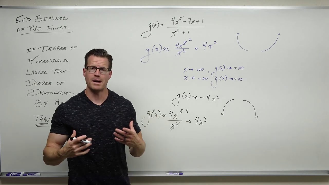
Finding End Behavior of Rational Functions (Precalculus - College Algebra 42)
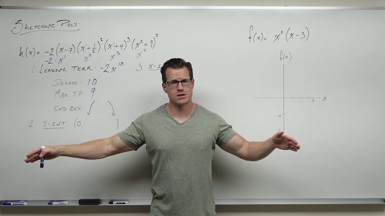
How to Sketch Polynomial Functions (Precalculus - College Algebra 31)
Ch. 3.2 Polynomial Functions and their Graphs
Power Functions (Precalculus - College Algebra 28)
5.0 / 5 (0 votes)
Thanks for rating: