5. Discrete Random Variables I
TLDRThis MIT OpenCourseWare lecture introduces the concept of random variables in probability theory, defining them as functions assigning numerical values to experimental outcomes. It explains discrete and continuous random variables, probability mass functions (PMFs), and the geometric PMF with examples. The lecture delves into expected value as an average value of a random variable and variance, which measures the spread of a distribution. It also covers properties of expectations, including linearity and effects of linear transformations on variance, providing foundational knowledge for further study in probability and statistics.
Takeaways
- 📚 The lecture introduces the concept of random variables in probability theory, explaining how they assign numerical results to outcomes of an experiment.
- 📈 Random variables are described using probability mass functions (PMFs), which assign probabilities to different numerical values that the variable can take.
- 🔢 The expected value of a random variable is a key concept, representing an average value that the variable can take, calculated by multiplying each value by its probability and summing these products.
- 📉 The concept of variance is also introduced, which measures the spread of a random variable's distribution, indicating how much the values deviate from the mean on average.
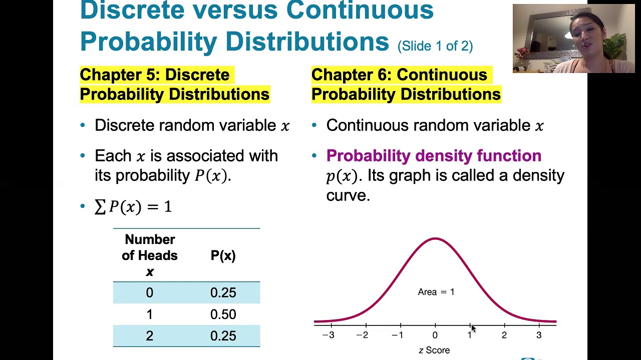
- 📊 Random variables can be discrete or continuous, with discrete variables taking on a countable number of values and continuous variables having an infinite range of possible values.
- 🎲 The lecture provides examples of calculating PMFs, such as the number of coin tosses until the first head appears, illustrating the geometric PMF.
- 🧩 The distinction between a random variable and its numerical values is emphasized, with the random variable being a function from the sample space to real numbers, while the numerical values are the outcomes of that function.
- 🔄 Functions of random variables are also random variables, as demonstrated by converting height from inches to centimeters, which is a function of the original height random variable.
- 📚 The importance of understanding discrete random variables before tackling continuous ones is highlighted, as the latter involves more complex mathematics including calculus.
- 📉 The properties of expected values are discussed, including how they relate to linear functions of random variables and the caution that the average of a function is not the same as the function of an average.
- 🔍 The variance is calculated using a shortcut formula that involves the expected value of the random variable and its square, providing a measure of dispersion around the mean.
Q & A
What is the main concept introduced at the beginning of the lecture?
-The main concept introduced at the beginning of the lecture is the concept of random variables. Random variables are ways of assigning numerical results to the outcomes of an experiment, which adds depth to the subject of probability theory.
What is the significance of defining random variables in probability theory?
-Defining random variables is significant because it allows for the assignment of numerical values to outcomes of an experiment, which can then be described using probability mass functions. This makes it possible to capture the likelihood of different numerical values occurring.
How are random variables represented in a compact way?
-Random variables are represented in a compact way using probability mass functions (PMFs). PMFs provide a method to describe the probability of a random variable taking on specific numerical values.
Can you provide an example of how a random variable is used in the context of an experiment?
-An example given in the lecture is the height of a random student. The experiment involves selecting a student at random and measuring their height, which assigns a numerical value (height in inches) to the outcome of the experiment.
What is the mathematical representation of a random variable?
-Mathematically, a random variable is represented as a function from the sample space into the real numbers. It takes an outcome of the experiment as an argument and produces a numerical value, which is the height of a particular student in the given example.
How is the concept of expected value of a random variable introduced?
-The concept of the expected value is introduced as a kind of average value of the random variable. It is a central concept in understanding the behavior of random variables over a large number of experiments.
What is the difference between a discrete and a continuous random variable?
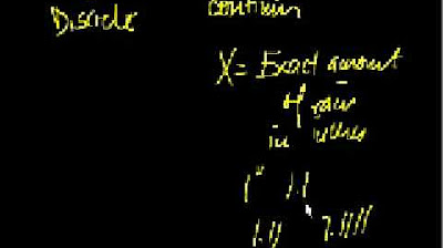
-A discrete random variable takes on a countable number of values, often integers (like the number of times heads appears when flipping a coin). A continuous random variable, on the other hand, can take on any value within an interval (like the height of a student measured to an infinite precision).
Why is it important to distinguish between the random variable itself and the numerical values it takes?
-It is important to distinguish between the random variable itself and the numerical values it takes because the random variable is a function that maps outcomes to numerical values, whereas the numerical values are the actual outcomes of the experiment. This distinction helps avoid confusion and conceptual errors in probability theory.
How is the probability mass function (PMF) of a random variable defined mathematically?
-The PMF of a random variable is defined mathematically as the probability that the random variable takes on a particular numerical value. It is calculated by summing the probabilities of all outcomes that lead to that specific numerical value.
Can you explain the concept of variance in the context of a random variable?
-Variance is a measure of how spread out the distribution of a random variable is. It is calculated as the expected value of the squared deviation from the mean. A high variance indicates that the values are spread out over a wide range, while a low variance indicates that they are concentrated close to the mean.
Outlines
📚 Introduction to Random Variables and Probability Theory
This paragraph introduces the concept of random variables in the context of probability theory. It explains that random variables assign numerical values to outcomes of experiments, making the subject more interesting and complex. The paragraph discusses how to define and describe random variables using probability mass functions (PMFs), which assign probabilities to different numerical outcomes. The speaker also mentions the importance of understanding the new concept of expected value and briefly touches on the concept of variance, setting the stage for the topics that will be covered in the unit.
🔢 Understanding Random Variables and Their Numerical Values
The speaker delves deeper into the concept of random variables, emphasizing their nature as functions mapping from the sample space to real numbers. Using the example of measuring the height of a student, the paragraph illustrates how numerical values are assigned to each outcome. It distinguishes between the random variable as an abstract function (denoted by a capital letter) and the specific numerical values it can take (denoted by lowercase letters). The paragraph also introduces the idea that multiple random variables can be derived from a single experiment, such as height and weight of a student, and discusses how functions of random variables are also random variables themselves.
📈 The Concept and Types of Random Variables
This paragraph further explores the concept of random variables, discussing their types, which can be discrete or continuous. The speaker uses the example of measuring height in inches versus a more precise scale to illustrate discrete and continuous random variables, respectively. The importance of understanding discrete random variables before moving on to continuous ones is highlighted, as the latter introduces complexities of calculus. The paragraph also emphasizes the distinction between the random variable itself and the numerical values it takes, using the notation of capital letters for variables and lowercase for specific values.
📊 Probability Mass Functions (PMFs) and Their Properties
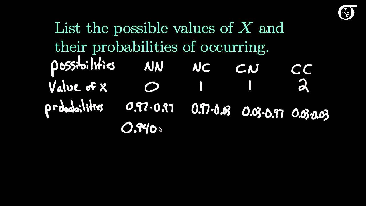
The speaker introduces PMFs as a way to describe the likelihood of different numerical values that a random variable can take. PMFs are represented as a bar graph where the height of each bar corresponds to the probability of the random variable taking on a particular value. The paragraph explains how to calculate PMFs by summing the probabilities of all outcomes that lead to a specific numerical value. It also provides an example of a geometric PMF, which describes the probability of the number of coin tosses until the first head appears, and discusses the properties of PMFs, such as all probabilities being non-negative and their sum equaling one.
🎲 Examples of Calculating PMFs for Discrete Random Variables
The paragraph provides examples of calculating PMFs for discrete random variables, using the scenarios of coin tossing and dice rolling. It explains how to determine the probability of a random variable taking a specific value by considering all possible outcomes that result in that value. The speaker illustrates this with a detailed example of rolling a tetrahedral die twice and calculating the PMF for the minimum value obtained. The concept of a geometric random variable is also revisited, with an emphasis on the calculation of PMFs for such variables.
📉 The Central Limit Theorem and the Shape of PMFs
The speaker discusses the Central Limit Theorem, a fundamental concept in probability theory, which states that the distribution of the sum (or average) of a large number of independent and identically distributed variables approaches a normal distribution, regardless of the original distribution. This is illustrated by plotting the PMF of the number of heads obtained in a series of coin tosses and observing how it begins to resemble a bell curve as the number of tosses increases. The paragraph also emphasizes the importance of understanding the PMFs of discrete random variables before tackling more complex continuous random variables.
🧮 The Expected Value: A Key Concept for Random Variables
This paragraph introduces the expected value of a random variable, which is a central concept in probability theory. The expected value is described as an average of the possible outcomes, weighted by their probabilities. The speaker provides an example using a game with different rewards and probabilities to illustrate the calculation of expected value. The paragraph also offers an alternative interpretation of expected value as the center of gravity of the distribution, which can be used to quickly calculate it in some cases, such as symmetric distributions.
🔄 Calculating Expected Values of Functions of Random Variables
The speaker explains how to calculate the expected value of a function of a random variable, using the law of the unconscious statistician. This law allows for the calculation of the expected value of a function by considering the original random variable's PMF, rather than finding the PMF of the function itself. The paragraph provides a mathematical justification for this law and highlights the importance of understanding when it is appropriate to apply this shortcut in calculations. It also includes a cautionary note that the average of a function of a random variable is not generally the same as the function of the average.
📉 Properties and Linearity of Expectations
This paragraph discusses the properties of expectations, particularly their linearity. It explains that the expected value of a linear function of a random variable is equal to the linear function of the expected value. The speaker provides examples, such as multiplying a random variable by a constant or adding a constant to a random variable, and demonstrates how these operations affect the expected value. The paragraph also emphasizes that while expectations are generally averages, the function of an average is not the same as the average of the function, except in the case of linear functions.
📊 The Variance: A Measure of Spread in Random Variables
The speaker introduces variance as a measure of how spread out the distribution of a random variable is. Variance is defined as the expected value of the squared deviation from the mean and gives more weight to larger deviations due to the squaring operation. The paragraph explains how to calculate variance using a practical formula that involves the expected value of the random variable and the expected value of its square. It also discusses the properties of variance, such as its non-negativity and how it changes under linear transformations, specifically that multiplying a random variable by a constant increases the variance by the square of that constant.
🔚 Conclusion on Variance and Linear Transformations
In the final paragraph, the speaker concludes the discussion on variance and its behavior under linear transformations. It reiterates that multiplying a random variable by a constant affects the variance by increasing it by the square of that constant, while adding a constant to a random variable does not change its variance. The paragraph wraps up the session and informs the audience that the next meeting will be on Wednesday.
Mindmap
Keywords
💡Random Variable
💡Probability Mass Function (PMF)
💡Expected Value
💡Variance
💡Discrete Random Variable
💡Continuous Random Variable
💡Sample Space
💡Geometric PMF
💡Law of the Unconscious Statistician
💡Linearity of Expectation
Highlights
Introduction of a new unit on probability theory focusing on random variables.
Definition of random variables as numerical assignments to outcomes of an experiment.
Explanation of probability mass functions (PMFs) to represent likelihoods of numerical values.
Illustration of how to calculate PMFs using examples of random variables.
Introduction of the concept of expected value as an average of a random variable.
Discussion on the variance of a random variable as a measure of spread.
Differentiation between discrete and continuous random variables.
Importance of understanding discrete random variables before tackling continuous ones.
Clarification on the distinction between a random variable and its numerical values.
Use of capital and lowercase letters to denote random variables and numerical values, respectively.
Calculation of PMFs by summing probabilities of outcomes leading to specific numerical values.
Example of calculating PMFs using a tetrahedral die toss experiment.
Illustration of the geometric PMF through a coin tossing experiment.
Introduction of the law of the unconscious statistician for calculating expected values.
Explanation of properties of expectations, including linearity and effects of constants.
Demonstration of how to calculate the expected value of a function of a random variable.
Caution against mistaking the average of a function of a random variable for the function of an average.
Introduction of variance as a measure of dispersion in a distribution.
Practical formula for calculating variance using expected values.
Properties of variance under linear transformations of random variables.
Transcripts
Browse More Related Video

Elementary Stats Lesson #9

Mathematical Statistics, Lecture 1
Introduction to Random Variables
Introduction to Discrete Random Variables and Discrete Probability Distributions

Session 40 - Probability Distribution Functions - PDF, PMF & CDF | DSMP 2023
6.1.1 The Standard Normal Distribution - Discrete and Continuous Probability Distributions
5.0 / 5 (0 votes)
Thanks for rating: