Probability Density Functions from Histograms
TLDRThis video tutorial guides viewers through the process of converting a histogram into a probability density function (PDF). It begins by explaining the concept of PDFs, using the normal distribution as a familiar example. The video then demonstrates how to scale the frequency of a histogram to create a PDF, ensuring the area under the curve equals one. The instructor uses a histogram of quiz scores as an example, adding a column to calculate the PDF values and adjusting the graph to represent the PDF. The video concludes by verifying the conversion's accuracy by summing the areas under the PDF graph, confirming that the total probability density equals one. A spreadsheet example is promised on the website for further exploration.
Takeaways
- 📚 The video explains how to convert a histogram into a probability density function (PDF).
- 📉 A histogram is a graphical representation of data frequency, while a PDF is a function that describes the likelihood of a random variable's possible outcomes.
- 🔢 The area under a PDF curve equals one, which is a key characteristic distinguishing it from a histogram.
- 📈 The normal distribution, also known as the Gaussian distribution or Bell curve, is a common example of a PDF.
- 🎓 High school students are likely familiar with the normal distribution and its properties, such as the 68% and 95% data points within one and two standard deviations, respectively.
- 📊 To convert a histogram into a PDF, a new column is added to the histogram table to represent the probability density.
- 🔑 The formula to calculate the probability density (P) is the frequency of the data divided by the total number of samples and the width of the bin.
- 📝 The video provides a step-by-step guide on how to adjust a histogram graph to represent a PDF, including changing the axis labels and plotting the data as s versus P.
- 📑 The presenter demonstrates the process using a histogram of quiz scores and shows how to scale the frequency to create a PDF.
- 🧩 To verify the conversion, the video shows how to calculate the total area under the PDF curve, which should equal one.
- 🔗 The video concludes with an offer to provide a copy of the spreadsheet used in the demonstration on the project's website.
Q & A
What is a probability density function (PDF)?
-A probability density function is a function that describes the likelihood of a continuous random variable taking on a particular value. Unlike histograms, the area under the curve of a PDF is equal to one, representing the total probability.
Why is the normal distribution also known as the Bell curve?
-The normal distribution is often referred to as the Bell curve due to its characteristic bell shape, which is symmetrical and centered around the mean.
What is the connection between the normal distribution and the Gaussian distribution?
-The normal distribution is also known as the Gaussian distribution, named after the physicist and mathematician Carl Friedrich Gauss, who made significant contributions to the study of these distributions.
What does the 68% rule in the context of the normal distribution signify?
-The 68% rule states that approximately 68% of the data in a normal distribution lies within one standard deviation of the mean.
How does the area under the curve of a probability density function relate to probability?
-The area under the curve of a probability density function represents the total probability, which must equal one for all possible outcomes of the random variable.
What is the process of converting a histogram into a probability density function?
-To convert a histogram into a probability density function, you scale the frequency counts by dividing them by the total number of samples and the width of the bins to ensure the area under the curve equals one.
Why is it necessary to divide by the number of samples and the bin width when converting a histogram to a PDF?
-Dividing by the number of samples and the bin width normalizes the histogram so that the total area under the resulting probability density function is one, which is a requirement for a PDF.
How can you verify that a histogram has been correctly converted into a probability density function?
-You can verify the conversion by summing the areas of the rectangles formed by the bins in the histogram. If the sum equals one, the conversion to a probability density function has been done correctly.
What is the significance of the vertical axis in a probability density function graph?
-The vertical axis in a probability density function graph represents the probability density at a given value of the random variable, not the frequency or count as in a histogram.
What is the role of calculus in understanding the area under the curve of a probability density function?
-Calculus is used to integrate the function over its entire domain to find the area under the curve, which should equal one for a valid probability density function.
Where can I find the spreadsheet mentioned in the video for further study?
-The spreadsheet can be found on the website for the project at Circle 4.com, biophysics. Look for the videos link near the top of the page.
Outlines
📊 Converting a Histogram to a Probability Density Function
This paragraph introduces the concept of converting a histogram into a probability density function (PDF). The speaker explains that PDFs are not as intimidating as they sound and that viewers are likely familiar with the normal distribution, often referred to as the Bell curve or Gaussian distribution. The importance of the area under the curve of a PDF being equal to one is highlighted, and the process of scaling frequency counts from a histogram to a PDF is outlined. The example of quiz scores is used to demonstrate how to add a column to the histogram table to represent the PDF, using a formula that divides the frequency by the total number of samples and the bin width. The speaker guides the viewer through the process of transforming a histogram graph into a PDF graph using Excel, emphasizing the need to ensure the area under the new graph equals one.
🔍 Validating the Probability Density Function Conversion
In this paragraph, the speaker focuses on validating the conversion of a histogram into a PDF. They discuss the need to ensure that the total area under the PDF graph represents a probability of one, which is done by summing the areas of rectangles formed by the histogram's bins. The speaker uses Excel to calculate the area under each step of the histogram, multiplies it by the bin width, and then divides by the number of occurrences to find the total area. The process is demonstrated step by step, and the speaker confirms that the sum of the areas equals one, indicating a successful conversion to a PDF. The speaker also mentions that a copy of the spreadsheet used in the demonstration will be made available on their website for further reference.
Mindmap
Keywords
💡Histogram
💡Probability Density Function (PDF)
💡Normal Distribution
💡Standard Deviation
💡Bell Curve
💡Gaussian Distribution
💡Area Under the Curve
💡Frequency
💡Bin
💡Calculus
💡Spreadsheet
Highlights
Introduction to converting a histogram into a probability density function (PDF).
Explanation of probability density functions and their relation to the normal distribution.
Historical context of the normal distribution being called the 'Bell curve' and 'Gaussian distribution'.
Description of the 68-95-99.7 rule related to standard deviations in the normal distribution.
Importance of the vertical axis in a PDF and its relation to probability.
The fundamental property of a PDF where the area under the curve equals one.
Conversion process from a histogram of scores to a PDF.
Adding a column to the histogram table to calculate the PDF.
Formula for scaling frequency to probability density using the number of samples and bin width.
Demonstration of how to apply the formula to the histogram data.
Using absolute reference in Excel to apply the formula to the entire table.
Method to transform a histogram graph into a PDF graph in Excel.
Explanation of changing the graph series to represent probability density versus score.
Verification of the correct calculation of PDF by summing the areas under the graph.
Final check to ensure the total probability density equals one.
Announcement of providing a spreadsheet on the website for further exploration.
Transcripts
Browse More Related Video
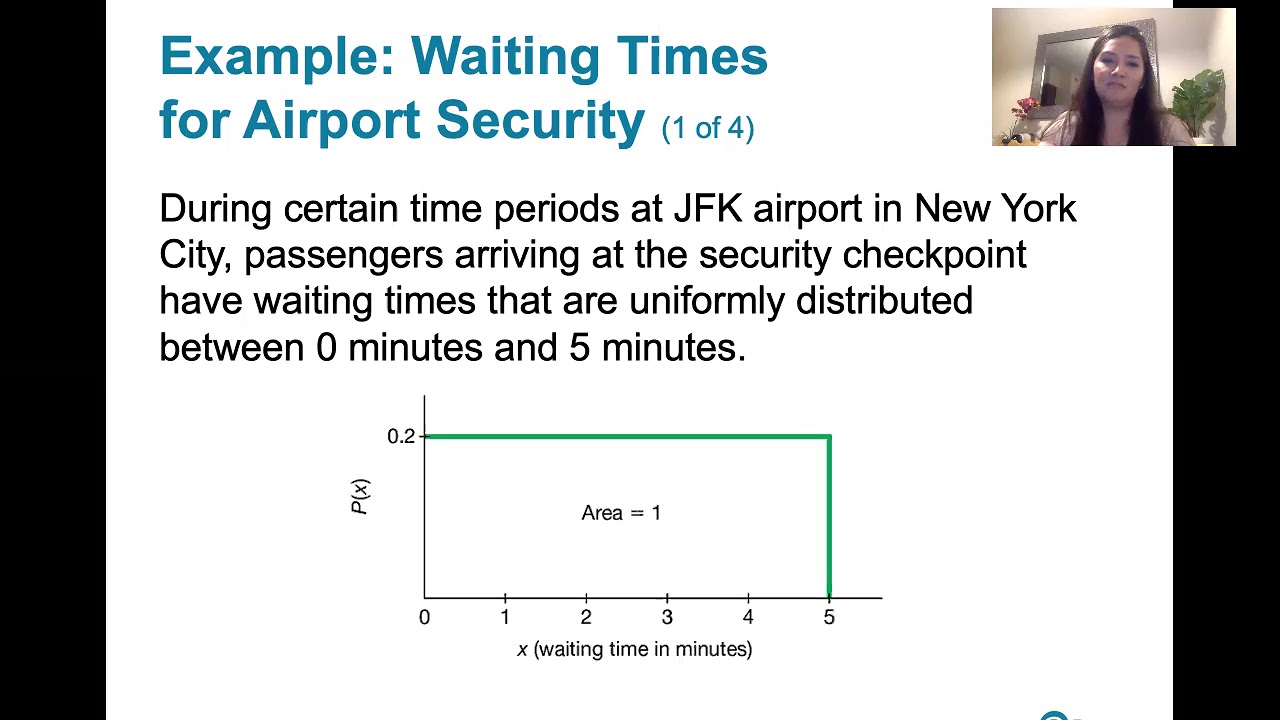
6.1.2 The Standard Normal Distribution - Uniform Distributions
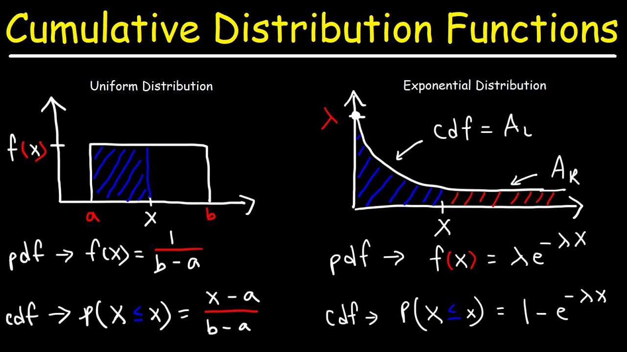
Cumulative Distribution Functions and Probability Density Functions
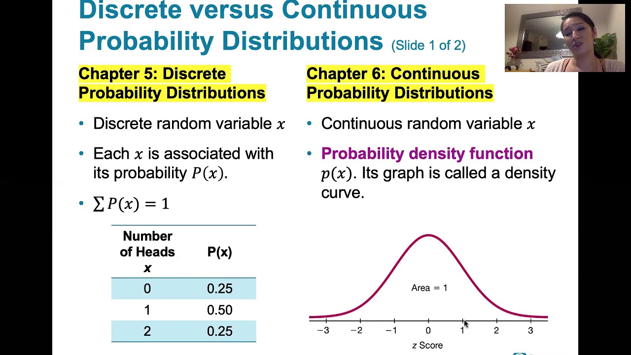
6.1.1 The Standard Normal Distribution - Discrete and Continuous Probability Distributions
Density Curves | Modeling data distributions | AP Statistics | Khan Academy

Why “probability of 0” does not mean “impossible” | Probabilities of probabilities, part 2
Probability Distribution Functions (PMF, PDF, CDF)
5.0 / 5 (0 votes)
Thanks for rating: