6.1.2 The Standard Normal Distribution - Uniform Distributions
TLDRThis video script explores uniform distributions in continuous probability, teaching viewers to graph and calculate probabilities for a range of values. It clarifies the role of the probability density function (PDF) and emphasizes that probabilities are determined by areas under the curve. The script uses a real-world example of waiting times at JFK airport, illustrating how to find the probability of waiting at least two minutes with a uniform distribution between zero and five minutes, highlighting the ease of calculating areas under a rectangular-shaped curve.
Takeaways
- 📚 The lesson focuses on uniform distributions, a type of continuous probability distribution where all values within a range are equally likely.
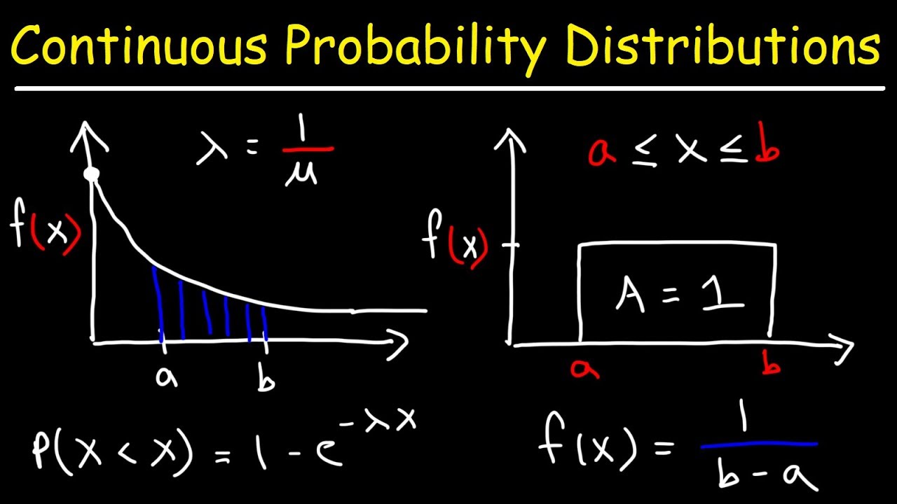
- 📈 To graph a uniform distribution, the probability density function (PDF) forms a rectangle, indicating the constant probability across the range of values.
- 📊 The PDF, represented by lowercase p(x), shows the probability per change in x, not the exact probability at a specific x value.
- 🌐 The area under the probability density curve represents the probability of a range of values, which is essential for continuous distributions.
- 🔢 For continuous distributions, probabilities are calculated by looking at areas under the curve, not at single points.
- 🎯 The total area under the curve for any continuous distribution must equal 1, representing the certainty that an event will occur.
- 📝 Uniform distributions are characterized by a constant probability density function, meaning the height of the rectangle in the graph is constant.
- ⏱ An example given in the script is the waiting times at JFK airport, which are uniformly distributed between 0 and 5 minutes.
- 📐 The height of the rectangle in a uniform distribution graph is calculated as 1 divided by the range of the distribution (e.g., 1/5 for a 0 to 5-minute range).
- 🤔 To find the probability of an event in a uniform distribution, such as waiting at least 2 minutes, you calculate the area of the relevant region under the curve.
- 🧩 The probability of waiting at least 2 minutes in the JFK example is found by multiplying the length of the time interval (3 minutes) by the height of the PDF (0.2), resulting in a 60% chance.
Q & A
What is a continuous random variable?
-A continuous random variable is a variable that can take on any value within a given range, as opposed to discrete random variables which can only take on specific values. It is associated with a probability density function (PDF) rather than a probability mass function.
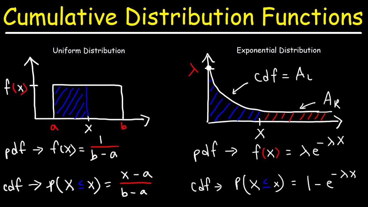
What is the difference between the probability density function (PDF) and the cumulative distribution function (CDF)?
-The probability density function (PDF), denoted as p(x), describes the probability per change in x and does not give the exact probability of a single value. In contrast, the cumulative distribution function (CDF), denoted as P(X ≤ x), gives the probability that the random variable X is less than or equal to a certain value.
How is the area under the probability density curve related to probabilities in continuous distributions?
-In continuous distributions, the area under the probability density curve (between two points) represents the probability that the random variable falls within that range. The total area under the curve is always equal to 1, representing the certainty that the random variable will take on one of its possible values.
What is a uniform distribution, and what does its graph look like?
-A uniform distribution is a type of continuous probability distribution where all possible values of the random variable are equally likely. The graph of a uniform distribution is a horizontal rectangle, with a constant height and the base covering the range of possible values.
How do you determine the height of the probability density function for a uniform distribution?
-For a uniform distribution, the height of the PDF is determined by ensuring that the area under the curve equals 1. The height is calculated as 1 divided by the range of the distribution (maximum value minus minimum value).
What is an example of a uniform distribution scenario mentioned in the script?
-An example given in the script is the waiting times of passengers at JFK airport in New York City, which are uniformly distributed between zero and five minutes.
How can you find the probability of a continuous random variable falling within a specific range in a uniform distribution?
-To find the probability, you calculate the area under the uniform distribution's curve within the specified range. This involves multiplying the width of the range by the constant height of the PDF.
What is the probability density function of a uniformly distributed random variable between 0 and 5 minutes?
-The probability density function for a uniformly distributed random variable between 0 and 5 minutes is p(x) = 1/5 for all x in the range [0, 5].
How do you interpret the probability of a passenger waiting at least two minutes at JFK airport, as given in the example?
-The probability of a passenger waiting at least two minutes is represented by the shaded area under the PDF from x=2 to x=5. In the example, this area is calculated to be 0.6, which means there is a 60% chance that a randomly selected passenger will wait two minutes or more.
Why is the total area under the PDF curve equal to 1 for any continuous probability distribution?
-The total area under the PDF curve is equal to 1 because it represents the certainty that the random variable will take on one of its possible values within the range. This is a fundamental property of probability distributions.
What is the significance of the term 'continuous' in 'continuous probability distribution'?
-The term 'continuous' signifies that the random variable can take on any value within an interval, and the probability is determined by the area under the PDF curve rather than discrete probabilities at specific points.
Outlines
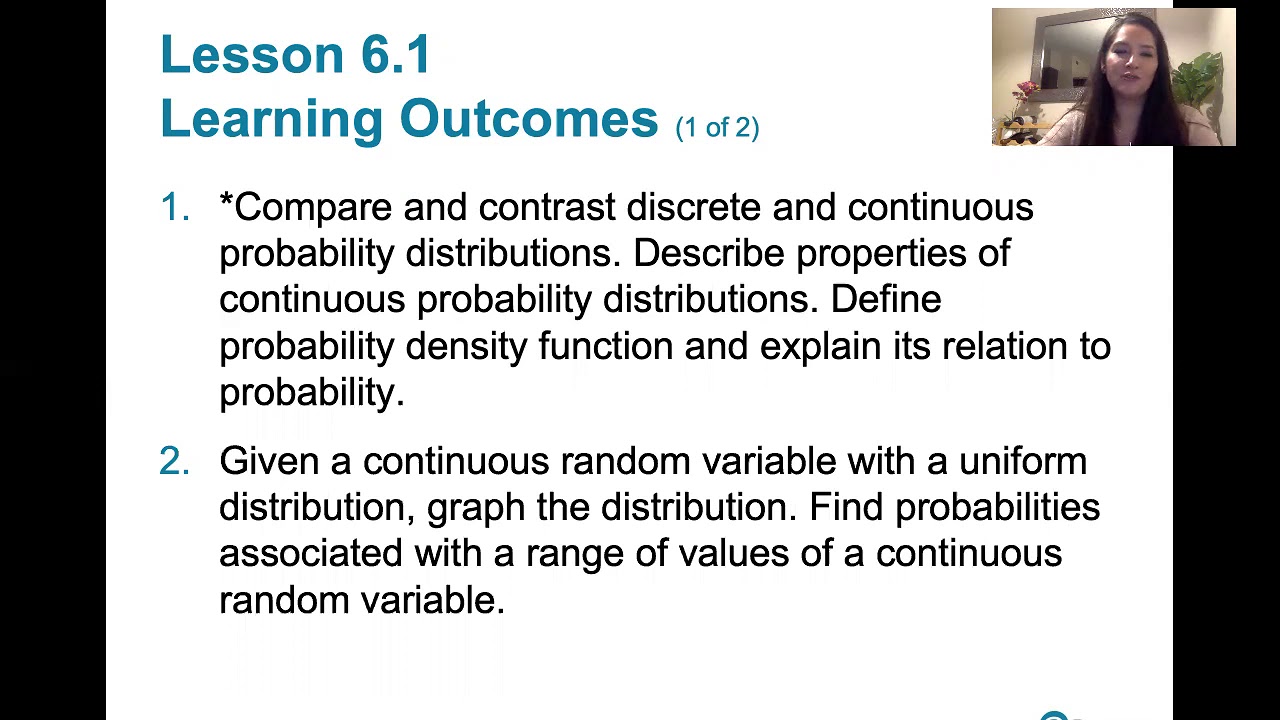
📈 Introduction to Uniform Distributions
This paragraph introduces the concept of uniform distributions in the context of continuous random variables. It explains that a uniform distribution is characterized by a constant probability density function (pdf), meaning all values within a certain range are equally likely. The video aims to teach viewers how to graph this distribution and calculate probabilities for ranges of values. The paragraph also outlines the general properties of continuous probability distributions, emphasizing that probabilities are represented by areas under the curve of the pdf, rather than the height of the curve itself. It sets the stage for a deeper dive into the uniform distribution and its applications, such as the example of waiting times at JFK airport being uniformly distributed between zero and five minutes.
📚 Properties and Calculation of Uniform Distributions
This paragraph delves into the specific properties of uniform distributions, illustrating how the probability density function remains constant across the range of possible values. It uses the waiting time at JFK airport as an example to explain how the constant height of the pdf is calculated as the reciprocal of the range (1/5 in this case) to ensure the total area under the curve equals one, representing a certainty of an event occurring. The paragraph then guides through a problem statement, showing how to calculate the probability of a randomly selected passenger waiting at least two minutes by shading the area corresponding to waiting times greater than or equal to two minutes and calculating the area as a simple rectangle multiplication, resulting in a 60% chance. This example solidifies the understanding of how areas under the uniform distribution curve correspond to probabilities.
Mindmap
Keywords
💡Uniform Distribution
💡Continuous Random Variable
💡Probability Density Function (PDF)
💡Probability Density Curve
💡Continuous Probability Distributions
💡Normal Distribution
💡Standard Normal Distribution
💡Area Under the Curve
💡Range
💡Probability
Highlights
The video discusses learning outcome number two from lesson 6.2, focusing on uniform distributions.
Uniform distributions are a type of continuous probability distribution where all possible values are equally likely.
Continuous random variables are described by a probability density function (pdf), notated as p(x), which represents probability per change in x.
The probability density function does not give the exact probability of a specific value but indicates the likelihood across a range.
Probabilities in continuous distributions are found by calculating areas under the probability density curve.
The total area under the probability density curve must equal one, representing the certainty that an event will occur.
Uniform distributions are characterized by a constant probability density function over a specified range.
The graph of a uniform distribution is rectangular, with the area under the curve representing probabilities.
Uniform distributions are used to model scenarios where all outcomes are equally likely within a range, such as waiting times at an airport.
The height of the uniform distribution's probability density function is calculated as 1 divided by the range of the variable.
An example given is the waiting times at JFK airport, which are uniformly distributed between zero and five minutes.
The probability density function for the JFK airport example is a constant value, ensuring the total area under the curve is one.
To find the probability of a waiting time of at least two minutes, the area under the curve from x=2 to x=5 is calculated.
The area calculation for the probability of waiting at least two minutes is a simple rectangle area computation.
The result of the area calculation gives a 60% chance of waiting two minutes or more, illustrating the practical application of uniform distributions.
The video aims to familiarize viewers with uniform distributions and their practical correspondence between areas and probabilities.
Uniform distributions are contrasted with normal distributions, which will be discussed in subsequent lessons.
The special case of the standard normal distribution is mentioned as a primary topic of a different lesson.
Transcripts
Browse More Related Video
Continuous Probability Distributions - Basic Introduction
Cumulative Distribution Functions and Probability Density Functions
6.1.0 The Standard Normal Distribution - Lesson Overview, Learning Outcomes
Probability density functions | Probability and Statistics | Khan Academy
Continuous Random Variables: Probability Density Functions
6.1.4 The Standard Normal Distribution - Given a range of z scores, find areas or probabilities.
5.0 / 5 (0 votes)
Thanks for rating: