Calculating the equation of a regression line | AP Statistics | Khan Academy
TLDRThis video script delves into the concept of bivariate data analysis, focusing on calculating the correlation coefficient and constructing the least squares regression line. It begins with a review of the correlation coefficient, emphasizing its role in determining the strength and direction of the relationship between two variables. The script then explains the process of deriving the equation for the regression line, highlighting the significance of the slope and y-intercept. Through a step-by-step calculation using a given dataset with a strong positive correlation (r=0.946), the video demonstrates how to calculate the slope as a product of the correlation coefficient and the ratio of standard deviations, and how to determine the y-intercept using the sample means. The final equation is presented as y hat = 2.50x - 2, offering a clear model for the data's trend.
Takeaways
- 📊 The script discusses the concept of calculating the correlation coefficient (r) for bivariate data, which measures the strength and direction of the relationship between two variables.
- 🔢 A perfect positive correlation is indicated by r=1, a perfect negative correlation by r=-1, and no correlation by r=0.
- 📈 The video introduces the process of deriving the equation for the least squares line, which aims to fit a set of data points as closely as possible.
- 📍 The script provides a visualization technique for understanding the data by plotting the sample mean and standard deviation for both x and y variables.
- 🔜 The slope (m) of the regression line is calculated as r multiplied by the ratio of the sample standard deviation of y to the sample standard deviation of x.
- 🅰️ The y-intercept (b) of the regression line is determined by ensuring the line passes through the point of sample mean of x and sample mean of y.
- 🤔 The script emphasizes the importance of understanding the intuitive reasoning behind the formulas used in regression analysis.
- 🏆 The example in the script yields an r of 0.946, indicating a strong positive correlation between the variables.
- 🧮 The calculation for the slope in the given example results in a value of approximately 2.50, and the y-intercept is determined to be -2.
- 📑 The final equation for the regression line in the example is written as y hat = 2.50x - 2, representing a best fit for the data points.
- 🎓 The video script serves as a comprehensive review and extension of statistical concepts related to bivariate data analysis and regression.
Q & A
What is the formula for the correlation coefficient?
-The formula for the correlation coefficient (r) is essentially the average of the product of the z scores for each pair of data points.
What does an r value of 1 indicate in correlation?
-An r value of 1 indicates a perfect positive correlation, meaning that the data points move in perfect tandem with each other as one variable increases, so does the other.
What does an r value of -1 indicate in correlation?
-An r value of -1 indicates a perfect negative correlation, which means that as one variable increases, the other decreases in a perfect inverse relationship.
What does an r value of 0 indicate in correlation?
-An r value of 0 indicates no correlation between the two variables, meaning that there is no linear relationship between the variables based on the data provided.
What is the equation for the least squares line?
-The equation for the least squares line is y-hat (the predicted y value) equals the slope (m) times x plus the y-intercept (b).
How is the slope (m) of the regression line calculated?
-The slope (m) of the regression line is calculated as r (the correlation coefficient) times the ratio of the sample standard deviation in the y direction over the sample standard deviation in the x direction.
How do you calculate the y-intercept (b) of the regression line?
-The y-intercept (b) can be calculated by using the point where the line crosses the y-axis, which is the sample mean of x and y (the point (x mean, y mean)). The formula to find b is y mean = m * x mean + b, and solving for b gives us the y-intercept.
What is the significance of the sample mean and standard deviation in plotting data points and the regression line?
-The sample mean and standard deviation are crucial for plotting data points and the regression line as they provide a measure of central tendency and dispersion for the data. They help in visualizing the spread of data points around the mean and how they relate to the regression line.
What would the regression line look like if r is 1?
-If r is 1, the regression line would have a slope equal to the standard deviation of y over the standard deviation of x, and it would pass through every point in the data set, showing a perfect positive linear relationship.
What would the regression line look like if r is -1?
-If r is -1, the regression line would have a slope that is the negative of the ratio of the standard deviation of y to the standard deviation of x, and it would have a perfect negative linear relationship with the data points, meaning for every unit increase in x, y would decrease by the same proportion.
What would the regression line look like if r is 0?
-If r is 0, the regression line would have a slope of 0, meaning there is no change in y as x increases. The line would be horizontal and pass through the point of the mean of x and y, showing no linear relationship between the variables.
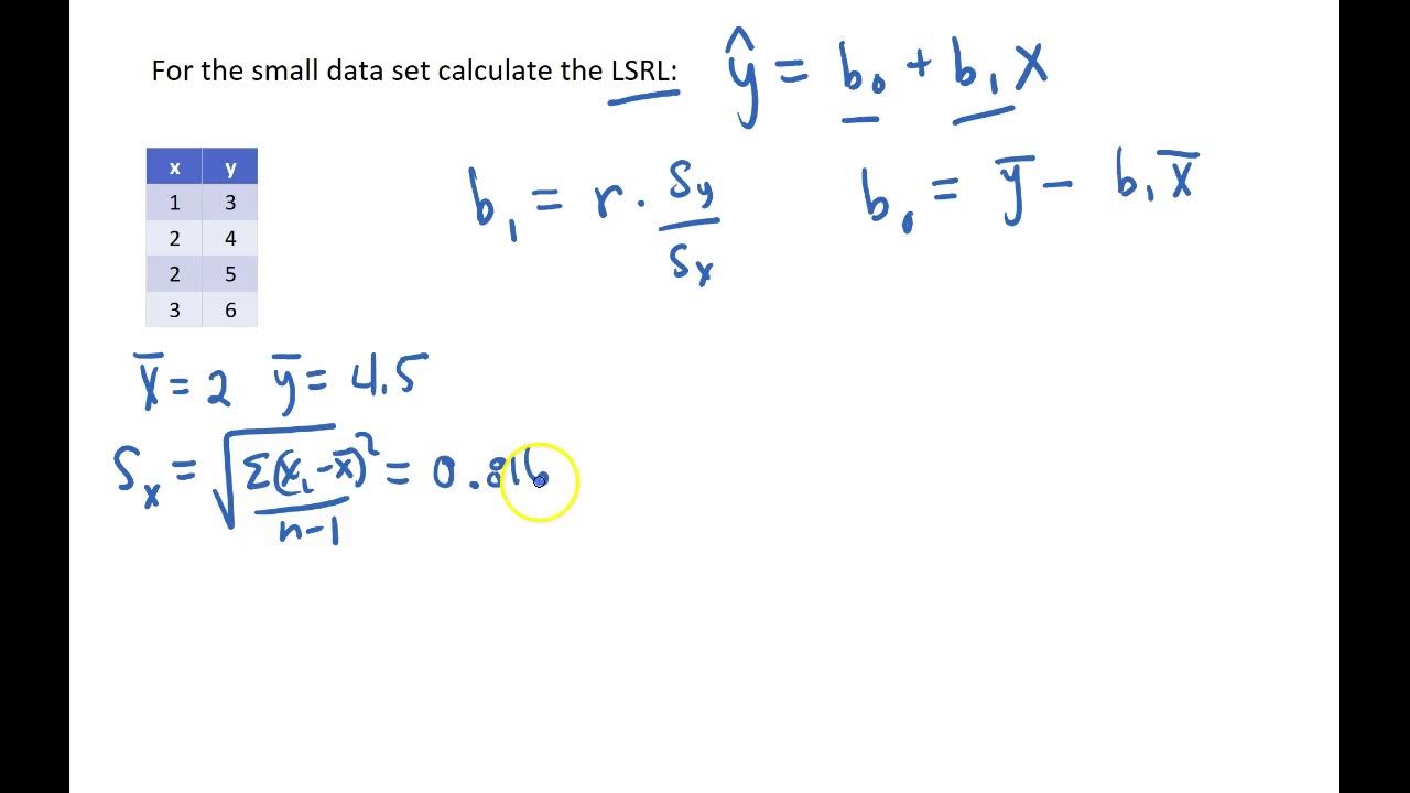
In the given dataset, what is the calculated slope (m) of the regression line?
-In the given dataset, the calculated slope (m) of the regression line is approximately 2.50, which is found by multiplying the correlation coefficient (0.946) by the ratio of the sample standard deviation of y (2.160) over the sample standard deviation of x (0.816).
What is the equation of the regression line for the provided dataset?
-The equation of the regression line for the provided dataset is y-hat = 2.50x - 2, where y-hat represents the predicted y values based on the x values.
Outlines
📊 Introduction to Bivariate Data Analysis
This paragraph introduces the concept of bivariate data analysis, focusing on the calculation of the correlation coefficient (r). It reviews the formula for calculating r, which is the average of the product of the z scores for each pair of data points. The discussion highlights that an r value of 1 indicates perfect positive correlation, -1 indicates perfect negative correlation, and 0 indicates no correlation. The example dataset has an r value of 0.946, indicating a strong positive correlation. The goal of this section is to derive the equation for the least squares line that fits these data points and to visualize the statistical concepts with a scatter plot of the data points, including the sample mean and standard deviation for both x and y variables.
📈 Deriving the Regression Line Equation
This paragraph delves into the process of deriving the equation for the least squares regression line, which is represented as y-hat = mx + b, where m is the slope and b is the y-intercept. The slope (m) is calculated as r times the ratio of the sample standard deviation in y to the sample standard deviation in x. The y-intercept (b) is determined by ensuring that the line passes through the point of sample mean of x and y. The paragraph provides an intuitive understanding of how the values of r affect the slope and the appearance of the regression line. It then applies this understanding to calculate the specific equation for the given dataset with an r value of 0.946, resulting in the equation y-hat = 2.50x - 2.
Mindmap
Keywords
💡bivariate data
💡correlation coefficient
💡z scores
💡least squares line
💡sample mean
💡sample standard deviation
💡slope
💡y intercept
💡perfect positive correlation
💡perfect negative correlation
💡no correlation
Highlights
The correlation coefficient (r) is explained as an average of the product of z scores for bivariate data pairs.
A perfect positive correlation is indicated by r equals one, perfect negative by r equals negative one, and no correlation by r equals zero.
The dataset discussed has a strong positive correlation with an r value of 0.946.
The video aims to derive the equation for the least squares line that fits the given data points.
Data points are visualized with their sample mean and standard deviation for better understanding.
The general form of a line equation is y = mx + b, where m is the slope and b is the y-intercept.
For regression lines, the slope (m) is calculated as r times the ratio of the standard deviation in y over the standard deviation in x.
The y-intercept (b) can be found by ensuring the line passes through the point of sample mean of x and y.
A perfect positive correlation (r=1) results in a line where the change in y equals the standard deviation of y over the standard deviation of x.
A perfect negative correlation (r=-1) is represented by a line with a slope of negative one.
When r is zero, the regression line is horizontal and passes through the mean of y only.
With a strong correlation like 0.946, the regression line closely fits the data points.
The slope (m) for the given dataset is calculated as 0.946 times the ratio of the standard deviations (2.160/0.816), resulting in approximately 2.50.
The y-intercept (b) is determined by the equation 3 = 2.50*2 + b, leading to b being -2.
The final equation for the regression line is y hat = 2.50x - 2.
The process of deriving the regression line equation is based on statistical principles and provides an intuitive understanding of the data fit.
The video emphasizes the importance of visualizing data statistics to build an intuition for the equation of the least squares line.
Understanding the relationship between r, standard deviations, and the resulting slope provides insight into how the data is spread across the x and y axes.
Transcripts


5.0 / 5 (0 votes)
Thanks for rating: