Elementary Stats Lesson #5
TLDRThis educational video script introduces the concept of bivariate data analysis, focusing on the relationship between two variables. It covers numerical summaries, scatter plots, and the linear correlation coefficient to determine the strength and direction of a linear relationship. The script uses real estate data as an example to demonstrate how to calculate the correlation coefficient manually and with a calculator, and how to derive the least squares regression line for predicting outcomes based on explanatory variables. It also discusses the importance of interpreting the slope and y-intercept in context and making predictions, setting the stage for further exploration of r-squared and other statistical concepts.
Takeaways
- 📚 The lesson focuses on analyzing bivariate data, which involves examining the relationship between two characteristics of the same individuals.
- 🏠 The primary example used in the lesson is the relationship between the size of a house and its selling price, with the aim to determine if larger houses tend to have higher selling prices.
- 📈 The lesson introduces the concept of explanatory and response variables, with size being the explanatory variable (x) and selling price being the response variable (y).
- 📊 To visualize the data, scatter plots are used, which help in identifying patterns and potential relationships between the two variables.
- 🔢 The lesson discusses the importance of calculating numerical summaries such as mean, standard deviation, and the correlation coefficient to quantify the relationship.
- 🔍 The correlation coefficient (r) measures the strength and direction of the linear relationship between two variables, with values ranging from -1 to 1.
- 📉 The direction of the linear relationship is determined by whether it is a positive or negative association; the strength is indicated by how close the correlation coefficient is to -1 or 1.
- 📚 The formula for calculating the correlation coefficient is provided, emphasizing its role in quantifying the linear relationship without being influenced by the units of measurement.
- ✂️ The concept of residuals is introduced, which are the differences between observed and predicted values, and are used to assess the fit of a linear model.
- 🧭 The least squares regression line (LSRL) is explained as the best fit line that minimizes the sum of squared residuals, providing the most accurate predictions for the response variable based on the explanatory variable.
- 🛠️ The use of technology, such as a calculator or computer, is highlighted for efficiently calculating the correlation coefficient and determining the LSRL for making predictions.
Q & A
What is the main focus of the lesson in the transcript?
-The main focus of the lesson is to analyze bivariate data, specifically looking at the relationship between two variables collected on the same group of individuals, and to describe that relationship using numerical summaries and graphical representations like scatter plots.
What is an 'explanatory variable' in the context of this lesson?
-An explanatory variable, denoted as 'x' in the lesson, is the variable that is thought to explain or influence the response variable to some extent. In the real estate example, the size of the house is the explanatory variable.
What is the 'response variable' in the context of the real estate example discussed in the lesson?
-The response variable, denoted as 'y', is the variable that is being explained or predicted by the explanatory variable. In the real estate example, the selling price of the house is the response variable.
What is a scatter plot and why is it used in this lesson?
-A scatter plot is a type of graphical representation used to display the relationship between two quantitative variables. It is used in this lesson to visualize the potential relationship between the size of a house and its selling price.
What is the formula for calculating the linear correlation coefficient (r)?
-The linear correlation coefficient (r) is calculated as the sum of the products of the standardized values of x and y (z-scores) divided by the degrees of freedom (n-1). The formula is complex and typically calculated with technology, but it essentially measures the strength and direction of the linear relationship between two variables.
What does the correlation coefficient (r) measure in the context of this lesson?
-The correlation coefficient (r) measures the strength and direction of the linear relationship between two quantitative variables. It ranges from -1 to 1, where values close to 1 or -1 indicate a strong linear relationship, and values close to 0 indicate a weak or no linear relationship.
Why is the least squares regression line (LSRL) important in analyzing bivariate data?
-The least squares regression line (LSRL) is important because it is the best-fit line that minimizes the sum of the squared residuals (the vertical distances between the data points and the line). It is used to make predictions about the response variable based on the explanatory variable.
How do you determine if a calculated correlation coefficient (r) indicates a strong linear relationship?
-A correlation coefficient (r) indicates a strong linear relationship if its absolute value is close to 1. The closer the value is to 1 or -1, the stronger the linear relationship. If r is close to 0, it suggests a weak or no linear relationship.
What is the purpose of calculating the least squares regression line for the real estate data in the lesson?
-The purpose of calculating the least squares regression line for the real estate data is to develop a model that can predict the selling price of a house based on its size. This model helps in understanding the influence of house size on selling price and can be used for future predictions.
How can the least squares regression line be used to predict the selling price of a house?
-The least squares regression line can be used to predict the selling price of a house by plugging the size of the house (x) into the line's equation, which results in a predicted selling price (y-hat). This prediction can then be used as an estimate, considering other market factors.
Outlines
📚 Introduction to Bivariate Data Analysis
The instructor begins by welcoming students to a new week of the semester and introduces the topic of bivariate data analysis, which involves examining the relationship between two characteristics of the same group of individuals. The focus is on numerical summaries and the use of scatter plots to visualize potential relationships. The example of a real estate agent studying the relationship between house size and selling price is used to illustrate the concept of explanatory and response variables.
📈 Scatter Plots and Data Visualization
The lesson continues with a detailed explanation of how to create scatter plots to visualize the relationship between two variables. The instructor guides students through the process of entering data into lists on a graphing calculator and using it to generate a scatter plot. The importance of graphing is emphasized as a preliminary step in understanding the data before delving into statistical analysis.
🔢 Descriptive Statistics for Bivariate Data
The instructor discusses the importance of calculating descriptive statistics for both variables in a bivariate dataset. The mean and standard deviation of house sizes and selling prices are calculated to understand the central tendency and dispersion of the data. This step is crucial for further analysis and for gaining insights into the data distribution.
📉 Exploring Linear Relationships
The focus shifts to identifying and understanding linear relationships between the two variables. The instructor explains the concept of positive and negative linear associations and how to interpret these relationships in the context of the data. The idea of a strong, moderate, or weak relationship is introduced, and the limitations of linear correlation in the presence of outliers are discussed.
🤔 Strength and Direction of Linear Associations
The instructor delves deeper into the measurement of the strength and direction of linear relationships using the linear correlation coefficient, denoted as 'r'. The formula for calculating 'r' is presented, and its properties are discussed, including its range from -1 to 1, its unitlessness, and its sensitivity to outliers. The concept of 'r' being specific to linear relationships is highlighted.
📊 Interpreting the Linear Correlation Coefficient
This section provides an interpretation guide for the linear correlation coefficient, explaining how values close to 1 or -1 indicate strong linear associations, while values near zero suggest a lack of linear relationship. The instructor uses scatter plots to visually demonstrate the strength of different associations and emphasizes the importance of this measurement in confirming observed patterns in the data.
🧮 Calculating the Correlation Coefficient
The instructor demonstrates the calculation of the correlation coefficient for the real estate data example, using the formula involving z-scores for both variables. The step-by-step process is shown, including standardizing the data, computing the products of the standardized values, and finding the sum. The calculated 'r' value confirms the strong positive linear association observed in the scatter plot.
🏠 Developing a Linear Model for Prediction
The lesson progresses to the development of a linear model to describe the relationship between house size and selling price. The instructor explains the importance of selecting a model that minimizes the sum of squared residuals, which are the differences between observed and predicted values. The concept of the least squares regression line as the best fit line is introduced.
📉 Methodologies for Linear Model Calculation
Two methods for calculating the least squares regression line are presented: the by-hand method using a formula with summary statistics, and the calculator method using technology for efficiency and accuracy. The instructor emphasizes the importance of using the best fit line for predictions and provides a formula for calculating the slope and y-intercept of the regression line.
🔍 Predicting Values Using the Regression Line
The instructor illustrates how to use the least squares regression line to make predictions, such as estimating the selling price of a house based on its size. The example of predicting the selling price for a 3,000 square foot house is used to demonstrate the application of the regression equation. The output from a calculator is also shown to highlight the ease and accuracy of technology in this process.
📝 Wrapping Up and Looking Forward
The instructor concludes the lesson by summarizing the key points covered, including the calculation of the correlation coefficient, the identification of linear patterns, and the use of the least squares regression line for predictions. An invitation for students to engage with the next lesson and assignment is extended, encouraging practice with the concepts learned.
Mindmap
Keywords
💡Bivariate Data
💡Explanatory Variable
💡Response Variable
💡Scatter Plot
💡Correlation Coefficient
💡Linear Association
💡Residuals
💡Least Squares Regression Line
💡R Squared (R²)
💡Critical Value
Highlights
Introduction to lesson five, chapter four, focusing on bivariate data analysis.
Utilization of numerical summaries to analyze relationships between two characteristics of data.
Explanation of bivariate data as involving two pieces of information or characteristics.
The concept of ordered pairs for representing individuals in a dataset.
Real estate example used to illustrate the relationship between house size and selling price.
Differentiation between explanatory variables (house size) and response variables (selling price).
Use of scatter plots to visualize the relationship between two variables.
Instructions on how to create scatter plots using a graphing calculator.
Analysis of average selling price and square footage in relation to the data distribution.
Investigation of linear relationships within bivariate datasets.
Description of positive and negative linear associations in data.
Introduction to the linear correlation coefficient as a measure of strength and direction of linear relationships.
Properties of the correlation coefficient, including its range from -1 to 1.
Explanation of how to calculate the linear correlation coefficient manually.
Use of technology to assist in calculating the correlation coefficient and least squares regression line.
Development of a linear model for predicting values based on the relationship between variables.
Method for determining the best-fit line using the least squares method.
Example of calculating the least squares regression line for real estate data.
Interpretation of the slope and y-intercept in the context of the real estate example.
Prediction of selling price for a 3000 square foot house using the regression line.
Demonstration of using a calculator to compute the least squares regression line and correlation coefficient.
Importance of diagnostics in calculators for obtaining additional statistical measures.
Application of regression analysis to lean body mass and metabolic rate data.
Explanation of how to determine if a correlation coefficient indicates a significant linear pattern.
Process of making predictions using the least squares regression line.
Assignment instructions for further practice with regression lines and correlation coefficients.
Transcripts
5.0 / 5 (0 votes)
Thanks for rating:


