Elementary Stats Lesson #6

walter dorman

31 Jan 202156:16

EducationalLearning

32 Likes 10 Comments

TLDRThis lesson delves into bivariate data analysis, focusing on the least squares regression line for predicting values based on a linear relationship. The instructor emphasizes understanding the formulas for slope and y-intercept rather than memorization, highlighting the importance of the correlation coefficient 'r' in determining linear association. The script guides through hand calculations and calculator methods for model generation, discusses the limitations of 'r', and introduces the concept of 'r-squared' as a measure of model effectiveness. The caution against extrapolation and the distinction between correlation and causation conclude the lesson, urging students to approach data analysis with critical thinking.

Takeaways

📚 The lesson continues the discussion on bivariate data, focusing on the least squares regression line for predicting 'y' values from given 'x' values.
🔍 Two methods for calculating the least squares regression line are introduced: by hand and using a calculator, emphasizing the importance of understanding the formulas rather than memorizing them.
📈 The correlation coefficient 'r' is pivotal, with values ranging from -1 to 1, indicating the strength and direction of a linear relationship between 'x' and 'y'.
🚫 A reminder that the correlation coefficient should not be overused and is only applicable for linear associations, not other types of relationships.
📊 The importance of constructing a scatter plot to visually assess the linear association before calculating 'r' is highlighted, along with using a critical value table to validate the linear relationship.
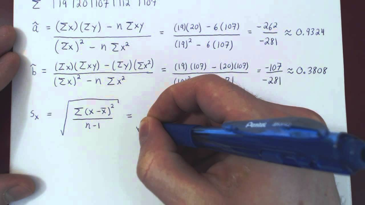
🧮 An example is provided to illustrate the manual calculation of the least squares regression line using given summaries like averages and standard deviations.
🤔 The script discusses the limitations of using the least squares regression line for predicting 'y' when the correlation coefficient is low, as in the example with parental income and child IQ.
🛠️ The calculator method for determining the least squares regression line is preferred for its ease and accuracy, demonstrated with a sample bivariate data set.
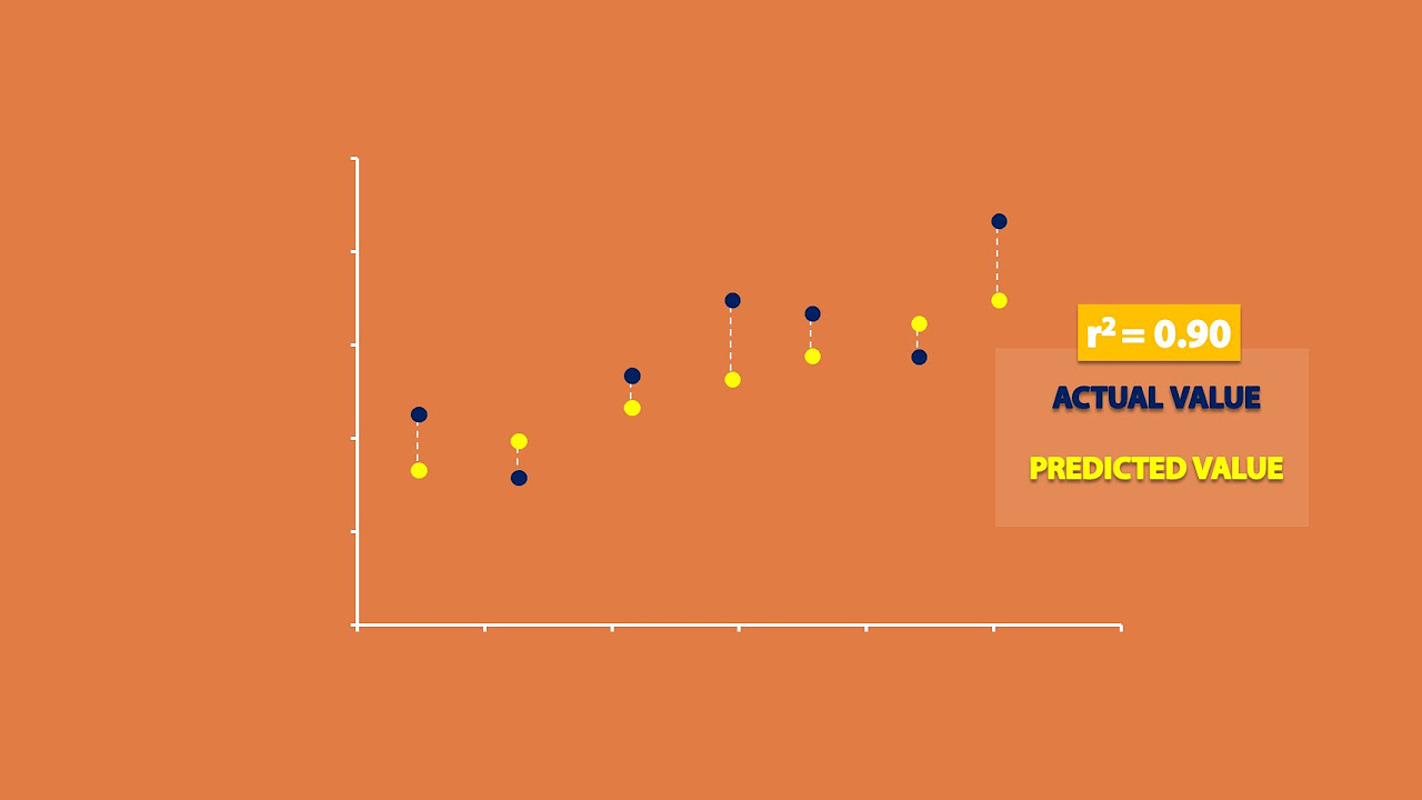
📉 The script introduces the concept of 'r-squared' as a measure of how well the regression line describes the relationship between 'x' and 'y', with a higher value indicating a better fit.
⚠️ A cautionary note is given against extrapolation, which is using the regression line to predict values outside the range of the collected data, as it can lead to unreliable predictions.
🔑 The coefficient of determination (r-squared) is key for understanding the quality of the model, indicating the proportion of the total variation from the average in 'y' that is explained by the model.

Q & A

What is the primary focus of the second half of chapter four in the textbook?
-The primary focus is on continuing the bivariate data discussion started in the previous lesson, specifically on the least square regression line and its application.
What are the two methods discussed for generating the least square regression line?
-The two methods discussed are the by-hand method, which involves manual calculations using certain summaries and formulas, and the calculator method, which uses a calculator to compute the regression line more efficiently.
What is the least square regression line used for?
-The least square regression line is used for predicting y values (y hat) from a given x value in a bivariate data set.
Why is it important to understand the formulas for the least square regression line rather than just memorizing them?
-It is important to understand the formulas to know what they are doing for you and how to utilize them effectively, rather than just memorizing them for the sake of a test or homework.
What is the correlation coefficient (r) and what is its range?
-The correlation coefficient (r) measures the strength and direction of the linear relationship between x and y. It ranges from -1 to 1, with -1 indicating a perfect negative linear relationship, 1 indicating a perfect positive linear relationship, and 0 indicating no linear relationship.
What is the purpose of constructing a scatter plot for bivariate data?
-A scatter plot is used to visually assess the linear association between x and y, which can then be verified by calculating the correlation coefficient (r).
What is the significance of the critical value in determining linear association?
-The critical value, found in table two, is used to determine if the absolute value of the correlation coefficient is significant enough to claim a linear association. If the absolute value of r is greater than the critical value, a linear association is confirmed.
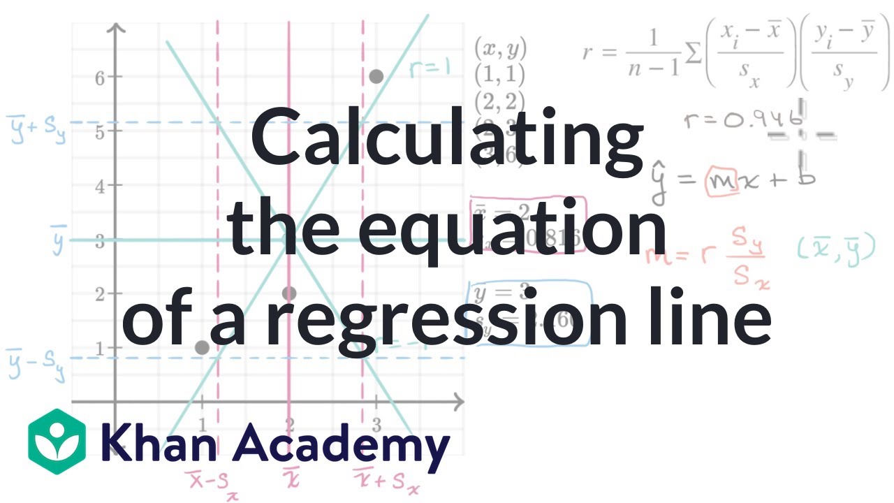
How is the slope (b1) of the least square regression line calculated in the by-hand method?
-The slope (b1) is calculated as the correlation coefficient (r) multiplied by the ratio of the standard deviation of y's to the standard deviation of x's.
What is the coefficient of determination (r squared) and how is it used?
-The coefficient of determination (r squared) measures the proportion of the total variation in the response variable that is explained by the least square regression line. It is used to assess the quality of the model and to compare different models.
Why is it incorrect to use the least square regression line for predicting values of x outside the range of the collected data?
-Using the least square regression line for predicting values of x outside the range of the collected data is incorrect because it is an act of extrapolation. The linear relationship may not hold outside the observed range, leading to unreliable predictions.
What is the difference between an observational study and a designed experiment?
-An observational study is one where responses are measured without any attempt to control for external factors, simply observing the data as it is. A designed experiment, on the other hand, uses randomization to control for possible external factors by randomly assigning individuals to explanatory values and observing the responses. Only designed experiments allow for the claim of causation.
What is a lurking variable or confounding variable, and why is it important in the context of correlation?
-A lurking variable or confounding variable is a factor that is related to both the explanatory and response variables and can affect the observed correlation. It is important because it can drive the changes seen in the data, making it difficult to determine causation. Only through a designed experiment with random assignment can confounding variables be controlled for.

Outlines

00:00

📚 Resuming Bivariate Data Discussion

The instructor continues the lesson on bivariate data analysis from the previous class, focusing on chapter four's second half. The aim is to further explore the concepts introduced earlier, specifically the least squares regression line for predicting y-values from given x-values. The importance of understanding the formulas for slope and y-intercept is emphasized, along with the reminder that these formulas will be provided and are not required to be memorized. The instructor also revisits the necessity of five summary statistics for manual calculation of the regression line and the significance of the correlation coefficient (r) in determining linear association, cautioning against its misuse outside of linear relationships.

05:00

🔍 Delving into Least Squares Regression Line Calculation

This section provides a step-by-step example of calculating the least squares regression line by hand, using the provided data on parental income and children's IQs. The instructor demonstrates how to derive the slope (b1) and y-intercept (b0) using the given averages, standard deviations, and the correlation coefficient. The calculated model is then used to predict a child's IQ based on a specific parental income. The instructor also discusses the limitations of this model, noting that a low r-value indicates a weak association and suggesting that other factors beyond parental income influence a child's IQ.

10:02

📈 Utilizing Technology for Regression Analysis

The instructor shifts the focus to using a calculator for regression analysis, starting with constructing a scatter plot from a given data set to visually assess the relationship between x and y. The correlation coefficient is calculated to verify the linear association suggested by the scatter plot. The least squares regression line is then derived using calculator functions, and the model's parameters, including the slope and y-intercept, are discussed. The r-squared value is introduced as a measure of how well the model fits the data, and a prediction is made using the derived model for a given x-value.

15:05

🤔 Questioning the Best Fit Model

The instructor poses a question about whether the least squares regression line is the best possible model for the data set, clarifying that while it is the best linear model, there may be other models, such as quadratic, that fit the data better. The concept of sum of squared residuals is introduced as a criterion for model fitness, and the instructor demonstrates how to use a calculator to perform quadratic regression, highlighting the improved fit of the quadratic model over the linear one.

20:06

📉 Understanding the Limitations of Correlation

This section discusses the limitations of the correlation coefficient, emphasizing that it only describes the strength and direction of a linear relationship and is not applicable to other types of relationships. The instructor also addresses the impact of outliers in bivariate data sets, referred to as influential points, which can significantly affect the slope and y-intercept of the regression line. The importance of calculating the regression line with and without influential points to understand their impact is highlighted.

25:08

⚠️ Avoiding Extrapolation in Predictions

The instructor warns against the practice of extrapolation, which is making predictions for x-values outside the range of the collected data. Using the real estate data example, the instructor demonstrates how using the regression model outside its valid range can lead to unreliable predictions. The importance of staying within the range of observed data when making predictions is emphasized to avoid erroneous results.

30:08

🔑 The Coefficient of Determination

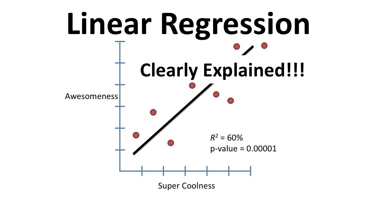
The instructor introduces the coefficient of determination (r-squared) as a measure of how well the regression line describes the relationship between x and y. It is calculated by squaring the correlation coefficient and represents the proportion of the total variation from the average in y that is explained by the regression line. The instructor illustrates this concept using the real estate data example, showing that 81% of the variation in selling price is explained by the square footage of the houses.

35:09

🚫 Correlation Does Not Imply Causation

The instructor concludes with a cautionary note about mistaking correlation for causation. Even with a high correlation coefficient, one cannot conclude that changes in x cause changes in y without a designed experiment. Observational studies can only indicate association, not causation. The instructor uses a hypothetical example involving shoe size and vocabulary aptitude in children to illustrate the absurdity of assuming causation from correlation and emphasizes the need for randomization in experiments to claim causation.

Mindmap

Keywords

💡Bivariate Data

Bivariate data refers to data sets that involve two variables, typically one independent variable (x) and one dependent variable (y). In the context of the video, bivariate data is central to the discussion of least squares regression analysis, where the relationship between two variables is explored to predict outcomes. The script uses bivariate data to illustrate the process of creating a least squares regression line, which is a fundamental concept in understanding the correlation and prediction between two variables.

💡Least Squares Regression Line

The least squares regression line is a straight line that best fits the data points on a scatter plot, minimizing the sum of the squares of the vertical distances of the points from the line. It is used for predicting y values from a given x value. The video script delves into the formula and calculation of this line, emphasizing its importance in statistical analysis for bivariate data sets, such as predicting a child's IQ based on parental income or house prices based on square footage.

💡Correlation Coefficient (r)

The correlation coefficient, denoted as 'r', is a measure that expresses the extent to which two variables are linearly related. It ranges from -1 to 1, with -1 indicating a perfect negative linear relationship, 1 indicating a perfect positive linear relationship, and 0 indicating no linear relationship. The script highlights the importance of the correlation coefficient in determining the strength and direction of the linear relationship between x and y in a bivariate data set.

💡Standard Deviation

Standard deviation is a measure of the amount of variation or dispersion in a set of values. In the script, the standard deviation for both x and y variables is mentioned as a necessary summary statistic for calculating the slope of the least squares regression line. It provides insight into the spread of the data points around the mean, which is crucial for understanding the variability within the data set.

💡Slope (b1)

The slope of a line, represented as 'b1' in the context of the script, indicates the steepness of the line and the direction of the relationship between x and y. A positive slope means that as x increases, y also increases, while a negative slope indicates an inverse relationship. The script explains how the slope is calculated using the correlation coefficient and the standard deviations of x and y, which is essential for determining the predictive power of the regression line.

💡Y-Intercept

The y-intercept is the point where the regression line crosses the y-axis. It is a key component of the regression equation and represents the expected value of y when x is zero. The script discusses how to calculate the y-intercept as part of the process of determining the least squares regression line, which is crucial for understanding the starting point of the predictive model.

💡Critical Value

A critical value is a value from a statistical table or distribution that is used to determine whether the observed correlation coefficient is significantly different from zero. The script mentions the use of a critical value table to assess whether the calculated correlation coefficient indicates a linear association that is statistically significant, which is an important step in validating the regression model.

💡R-Squared (R²)

R-squared, or the coefficient of determination, is a statistical measure that represents the proportion of the variance for a dependent variable that's explained by an independent variable or variables in a regression model. The script introduces R-squared as a way to evaluate the goodness of fit of the regression model, with a higher R-squared value indicating a better fit of the model to the data.

💡Outliers

Outliers are data points that are significantly different from other observations in a data set. In the context of bivariate data, outliers can be referred to as influential points, which can have a significant impact on the slope and y-intercept of the regression line. The script warns against the influence of outliers and suggests that they can skew the regression model, leading to less accurate predictions.

💡Extrapolation

Extrapolation is the process of predicting values of the dependent variable outside the range of the independent variable that was used to create the regression model. The script cautions against using the least squares regression line for extrapolation, as it can lead to unreliable predictions. This is because the linear relationship may not hold for values outside the observed data range.

💡Coefficient of Determination

The coefficient of determination, often represented as R², is a statistical measure that indicates how well a regression model fits a data set. It is calculated as the square of the correlation coefficient (R). The script explains that R² provides an indication of the percentage of variance in the dependent variable that is predictable from the independent variable(s). A higher R² value suggests a better fit of the model to the data, which is important for understanding the predictive power of the regression line.

💡Observational Study

An observational study is a type of research methodology where data is collected and analyzed without the researcher exerting any influence on the variables under study. The script points out that in observational studies, one can only identify correlations between variables but cannot infer causation. This is because there may be confounding variables that are related to both the independent and dependent variables, which could be driving the observed correlations.

💡Causation

Causation refers to a cause-and-effect relationship between variables, where a change in one variable leads to a change in another. The script emphasizes the distinction between correlation and causation, noting that while a strong correlation can be observed in an observational study, it does not imply that one variable causes the change in the other. Establishing causation typically requires a designed experiment with controlled conditions and randomization.

💡Designed Experiment

A designed experiment is a scientific study that involves manipulating one or more variables to determine whether changes in these variables cause changes in other variables. The script explains that designed experiments, unlike observational studies, allow researchers to claim causation by controlling for confounding variables through random assignment. This method is more rigorous and can provide evidence of a true cause-and-effect relationship between variables.

Highlights

Continuation of the bivariate data discussion from the previous lesson, focusing on the least squares regression line.

Introduction of two methods for calculating the least squares regression line: by hand and using a calculator.

Explanation of the importance of understanding the formulas for the least squares regression line rather than memorizing them.

Discussion on the five summaries necessary for generating the least squares regression line by hand.

Clarification that the correlation coefficient, r, is only used for linear association and its limitations.

Introduction of the concept of critical values for the correlation coefficient to claim linear association.

Example of calculating the least squares regression line by hand using data from a study on parental income and children's IQ.

Explanation of the limitations of the model in predicting children's IQ based on parental income due to a low r value.

Demonstration of using a calculator to find the least squares regression line and the importance of constructing a scatter plot first.

Process of calculating the correlation coefficient using a calculator and interpreting its value.

Introduction of the concept of R-squared as a measure of how well the regression line describes the relationship between variables.

Comparison of R-squared values for linear and quadratic models to determine which model fits the data better.

Discussion on the limitations of the correlation coefficient and its inability to describe non-linear relationships.

Caution against using the least squares regression line for extrapolation beyond the range of the data collected.

Explanation of the coefficient of determination and its role in indicating the quality of the model for prediction.

The difference between observational studies and designed experiments, and the importance of randomization in claiming causation.

Highlighting the danger of mistaking correlation for causation without proper experimental design.

Final thoughts on the importance of understanding the limitations of regression models and the need for proper study design.

Transcripts

Browse More Related Video

Elementary Stats Lesson #5

Calculating the equation of a regression line | AP Statistics | Khan Academy

Regression and R-Squared (2.2)

Linear Regression and Correlation - Example

Linear Regression, Clearly Explained!!!

Linear Regression, Clearly Explained!!!

Related Tags

Linear Regression Correlation Coefficient Statistical Analysis Bivariate Data Least Squares Predictive Modeling Data Interpretation Observational Study Causation Misconception Educational Tutorial