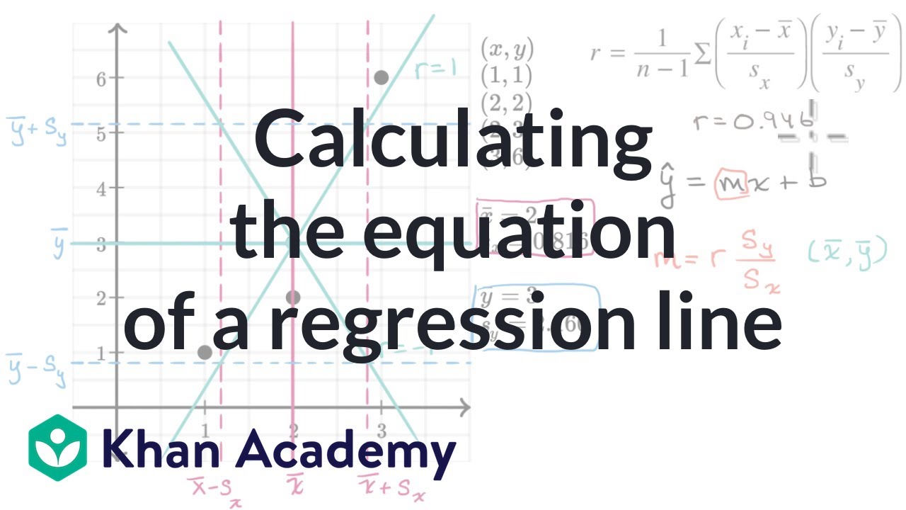
Calculating the Least Squares Regression Line by Hand
TLDRThe video script presents a step-by-step guide on calculating the least squares regression equation for a small dataset. It explains how to estimate the intercept (b0) and slope (b1) using the correlation coefficient (r), standard deviations (sy and sx), and averages (y-bar and x-bar). The example provided demonstrates the calculations, resulting in a slope value of approximately 1.5 and an intercept of 1.5, highlighting that this specific outcome is unusual but serves as a clear example of the process.
Takeaways
- 📊 The script explains the process of calculating the least squares regression equation for a small dataset.
- 🔢 The equation is in the form y-hat = b0 + b1x, where b0 is the intercept and b1 is the slope.
- 🧮 To find the slope (b1), use the formula b1 = r * sy / sx, where r is the correlation coefficient, sy is the standard deviation of y, and sx is the standard deviation of x.
- 📈 The intercept (b0) is calculated using b0 = y-bar - b1 * x-bar, with y-bar and x-bar being the averages of the y's and x's respectively.
- 🌟 The averages (y-bar and x-bar) are found by summing the values and dividing by the total number of observations.
- 📐 The standard deviations (sx and sy) are calculated using a formula involving the summation of squared differences from the mean, divided by n-1.
- 🤏 The script provides example values: x-bar equals 2, y-bar equals 4.5, sx equals 0.816, and sy equals 1.291.
- 🔗 The correlation coefficient (r) is given as 0.949, which is used to find the slope.
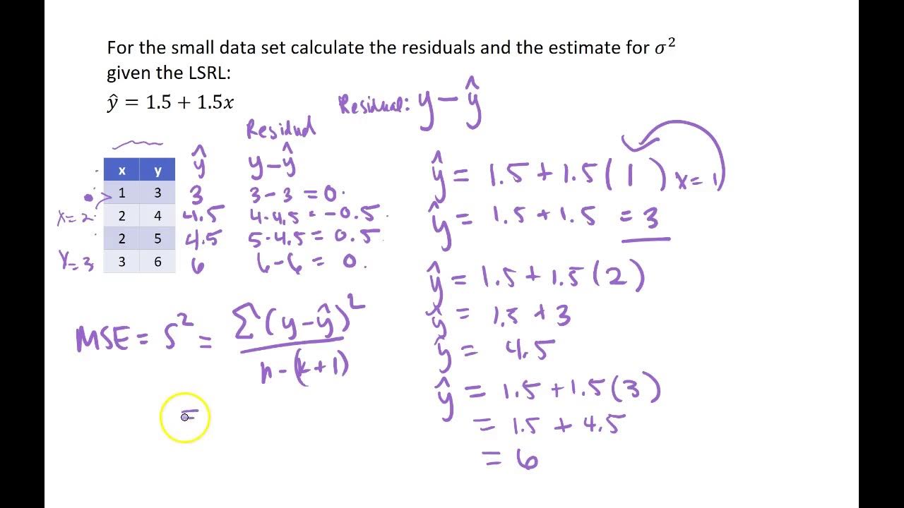
- 🧠 The calculated slope (b1) is approximately 1.5, and interestingly, the intercept (b0) also equals 1.5 in this specific example.
- 📝 The final least squares regression equation for the example is y-hat = 1.5 + 1.5x, highlighting that the slope and intercept coincidentally are the same in this case.
- 💡 This example serves as a clear, step-by-step guide on how to manually calculate the least squares regression line for a small dataset.
Q & A
What is the purpose of calculating the least squares regression equation?
-The purpose of calculating the least squares regression equation is to find the best-fit line that minimizes the sum of squared differences (residuals) between the observed values and the values predicted by the line. This line is used to model the relationship between two variables and make predictions.
What are the two main components of the least squares regression equation?
-The two main components of the least squares regression equation are the intercept (b0) and the slope (b1).
How can we calculate the slope (b1) of the regression line?
-The slope (b1) can be calculated using the formula b1 = r * sy / sx, where r is the correlation coefficient, sy is the standard deviation of y, and sx is the standard deviation of x.
What is the formula for calculating the intercept (b0) in the regression equation?
-The intercept (b0) can be calculated using the formula b0 = y-bar - b1 * x-bar, where y-bar is the average of y values and x-bar is the average of x values.
What are x-bar and y-bar in the context of the least squares regression?
-In the context of the least squares regression, x-bar and y-bar represent the mean or average values of the x and y data points, respectively. They are calculated by summing all the values in each set and dividing by the total number of data points.
How can we find the sample standard deviations for x and y?
-The sample standard deviations for x and y can be found by taking the square root of the sum of each observation minus its mean squared, divided by n minus 1, where n is the number of observations.
What is the correlation coefficient (r) in the context of regression analysis?
-The correlation coefficient (r) is a measure of the strength and direction of the linear relationship between two variables. It ranges from -1 to 1, where 1 indicates a perfect positive linear correlation, -1 indicates a perfect negative linear correlation, and 0 indicates no linear correlation.
How do you calculate the correlation coefficient (r) manually?
-To calculate the correlation coefficient (r) manually, you can use the formula: 1 over (n - 1) times the summation of (xi - mean of x) * (yi - mean of y) divided by the product of the standard deviation of x and the standard deviation of y.
What does it mean when the slope and intercept of a regression equation are the same?
-When the slope and intercept of a regression equation are the same, it is a peculiar occurrence that suggests a specific relationship between the x and y variables in the dataset. However, this is not a common situation and may be due to the particular characteristics of the data set being analyzed.
How can we use the calculated values of b0 and b1 to make predictions?
-Once the values of b0 (intercept) and b1 (slope) are calculated, they can be used to make predictions by substituting the value of x into the regression equation: y-hat = b0 + b1 * x. The result, y-hat, gives the predicted value of y for a given x.
What is the significance of the least squares regression equation in statistical analysis?
-The least squares regression equation is significant in statistical analysis as it provides a simple and effective method to model the relationship between two variables. It is widely used in various fields for forecasting, trend analysis, and decision-making processes based on the underlying relationship between variables.
Outlines
📊 Calculating the Least Squares Regression Equation
This paragraph introduces the process of calculating the least squares regression equation for a small data set. It explains the need to estimate the intercept (b0) and the slope (b1) of the equation y-hat = b0 + b1x. The paragraph outlines the steps to calculate these parameters manually, including the formulas for slope (b1 = r * sy / sx) and intercept (b0 = y-bar - b1 * x-bar), where r is the correlation coefficient, sy and sx are the sample standard deviations for y and x, respectively, and y-bar and x-bar are the averages of y and x. The paragraph provides an example with specific values for x-bar (2) and y-bar (4.5), and explains how to calculate the sample standard deviations for x (sx = 0.816) and y (sy = 1.291). It also mentions the previously calculated correlation coefficient (r = 0.949) and uses these values to demonstrate the calculation of the slope (b1 ≈ 1.5) and intercept (b0 = 1.5), noting that in this particular example, the slope and intercept happen to be the same, which is an unusual occurrence. The final equation derived is y-hat = 1.5 + 1.5x, representing the least squares regression line for the given data set.
Mindmap
Keywords
💡Least Squares Regression
💡Intercept (b0)
💡Slope (b1)
💡Correlation Coefficient (r)
💡Standard Deviation
💡Average (Mean)
💡Calculation
💡Data Set
💡Regression Equation
💡Hand Calculation
💡Observation
Highlights
Calculation of the least squares regression equation is discussed using a small data set.
The equation for the regression line is y hat = b0 + b1x, where b0 is the intercept and b1 is the slope.
The method to estimate the intercept (b0) and slope (b1) is explained through a step-by-step process.
The formula for calculating the slope (b1) is given as b1 = r * sy / sx, where r is the correlation coefficient, sy is the standard deviation of y, and sx is the standard deviation of x.
The formula for the intercept (b0) is derived as b0 = y-bar - b1 * x-bar, with y-bar and x-bar being the averages of y and x values respectively.
The calculation of averages for x and y values is explained by summing them up and dividing by the total count.
The concept of sample standard deviation is introduced with a formula for its calculation.
The standard deviation for x (sx) is calculated to be 0.816.
The standard deviation for y (sy) is determined to be 1.291.
The correlation coefficient (r) is calculated to be 0.949, which is used in the formula for the slope.
The actual calculation of the slope (b1) results in a value of approximately 1.5.
The intercept (b0) is calculated and found to be equal to the slope, which is 1.5, in this particular example.
The final form of the least squares regression equation is provided as y-hat = 1.5 + 1.5x.
The process is demonstrated to be reproducible and can be done by hand for small data sets.
The example serves as a clear guide for those learning the fundamentals of regression analysis.
The transcript provides a comprehensive understanding of the statistical concepts involved in regression analysis.
The practical application of the calculations is emphasized, making the content relevant to real-world scenarios.
The discussion includes the importance of understanding the underlying formulas and their components.
The transcript is a valuable resource for anyone seeking to understand the basics of least squares regression.
Transcripts
Browse More Related Video


5.0 / 5 (0 votes)
Thanks for rating: