Avon High School - AP Calculus BC - Topic 10.12 - Example 1

Tony Record

7 Mar 202120:30

EducationalLearning

32 Likes 10 Comments

TLDRThis transcript delves into the Lagrange error bound, a concept used to determine the accuracy of approximations made using Taylor or Maclaurin polynomials. The video explains the motivation behind studying this topic, the interchangeability of the terms 'remainder' and 'error', and how the error bound is calculated using the nth plus 1 derivative of a function. It also touches on the historical significance of Lagrange in calculus and provides an example to illustrate the application of the Lagrange error bound in approximating the sine function. The video emphasizes the importance of understanding and practicing these concepts to ensure accurate and reliable approximations.

Takeaways

📚 The Lagrange error bound is a complex topic often studied in calculus to understand how close approximations are to the actual values of functions.
🔍 The motivation for studying the Lagrange error bound comes from the need to determine the reliability of approximations made using Taylor or Maclaurin polynomials.
🤔 The remainder (error) is the difference between the actual value of the function and its approximated value, with absolute values taken for the comparison.
📈 Taylor's theorem and the Lagrange error bound are powerful when combined, allowing for the inclusion of a remainder term in the approximation to account for accuracy.
📊 The remainder is defined as the (n+1)th derivative of the function evaluated at some point z, multiplied by (x-c)^(n+1) and divided by (n+1)!, all in absolute values.
🤷‍♂️ The specific value of z (between x and c) is often elusive and not necessary to find, as it can be circumvented by finding the maximum value of the (n+1)th derivative.
👨‍💼 Joseph Lagrange, a key figure in calculus, introduced the prime notation for derivatives and was instrumental in the development of calculus and series.
🧮 The nth plus one derivative term is used to find an error bound, which is the maximum possible error and can be considered as the worst-case scenario.
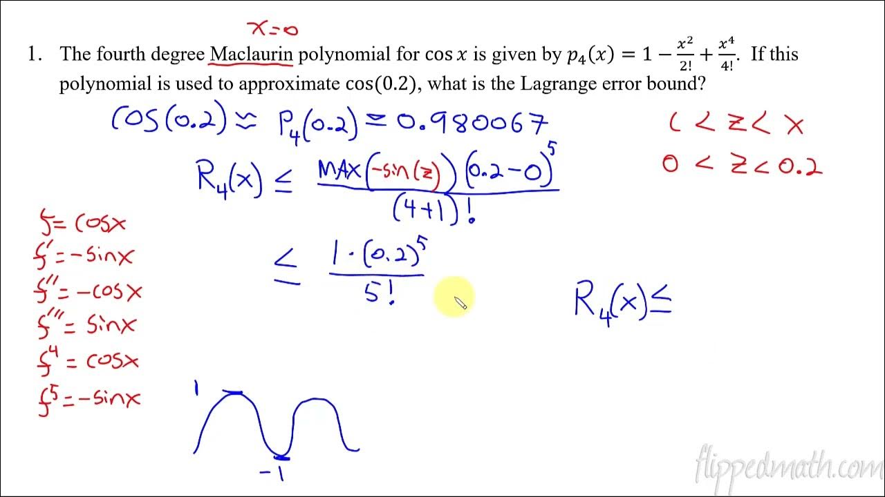
📐 In the provided example, the third degree Maclaurin polynomial for the sine function of x is used to approximate the sine of 0.1 and determine its accuracy.
🔢 The actual error is calculated by finding the absolute value of the difference between the actual sine of 0.1 and the approximation given by the third degree polynomial.
📝 The process of finding the Lagrange error bound and the actual error involves both theoretical calculations and practical approximations, highlighting the importance of practice and immersion in the material.

Q & A

What is the main topic of the transcript?
-The main topic of the transcript is the Lagrange error bound, which is used to determine the accuracy of approximations made using Taylor or Maclaurin polynomials.
Why is it important to study the Lagrange error bound?
-Studying the Lagrange error bound is important because it helps us understand how close the approximations made with Taylor or Maclaurin polynomials are to the actual value of the function, allowing us to determine if the approximations are reliable enough for practical use.
What does the term 'remainder' refer to in the context of the transcript?
-In the context of the transcript, 'remainder' refers to the error or the difference between the actual value of the function and its approximated value using a polynomial.
What is the role of the variable 'z' in the Lagrange error bound expression?
-The variable 'z' in the Lagrange error bound expression is a value that lies between the point 'c' (the center of the polynomial) and 'x' (the point at which the function is being approximated). It is used to evaluate the nth plus 1 derivative of the function, which contributes to determining the error bound.
How does one deal with not knowing the exact value of 'z'?
-If the exact value of 'z' is not known, one can estimate the maximum value of the nth plus one derivative over the interval containing 'c' and 'x'. This estimation is used to find an upper bound for the remainder, which serves as the error bound.
Who was Lagrange and why is he significant in calculus?
-Lagrange was a prominent mathematician who made significant contributions to the development of calculus, particularly in the areas of series and derivatives. He is renowned for introducing the prime notation for derivatives for the first time.
What is the third degree Maclaurin polynomial for the sine function?
-The third degree Maclaurin polynomial for the sine function is given by p3(x) = x - x^3/3!. In this case, it is used to approximate the sine of 0.1.
How is the accuracy of the approximation using the third degree Maclaurin polynomial determined?
-The accuracy is determined by using Taylor's theorem and the Lagrange error bound. By calculating the maximum of the fourth derivative of the function (sine in this case) and applying the error bound formula, one can estimate the maximum possible error.
What is the actual error in approximating the sine of 0.1 using the third degree Maclaurin polynomial?
-The actual error is the absolute value difference between the actual sine of 0.1 and the approximation given by the third degree Maclaurin polynomial. The calculated error was found to be much smaller than the estimated error bound, indicating a high degree of accuracy.
What advice does the speaker give regarding the study and application of the Lagrange error bound?
-The speaker advises that understanding and applying the Lagrange error bound requires practice and immersion in the material. They emphasize that it may not make immediate sense after watching a video or two, but with dedicated practice, the concepts will become clearer.

Outlines

00:00

📚 Introduction to Lagrange Error Bound

The paragraph begins with a welcome back to students and introduces the topic of Lagrange error bound, which is considered complex but will be explained in a way that minimizes its intimidating reputation. The discussion shifts to the motivation behind studying this topic, which is to understand the accuracy of approximations made using Taylor and Maclaurin polynomials. The concept of 'remainder' and 'error' is introduced as interchangeable terms, with the remainder being the difference between the actual and approximated values of a function. The lesson aims to clarify these concepts and their significance in approximating functions.

05:01

🔢 Historical Context and Theoretical Foundation

This paragraph delves into the historical significance of Lagrange in the field of calculus, highlighting his contributions and collaborations with Leonard Euler. It addresses the challenge of finding the 'z' value in the Lagrange error bound formula, emphasizing that while it may seem important, it is often not necessary to pinpoint 'z'. The approach to handling the unknown 'z' involves estimating the maximum value of the nth plus one derivative, which provides an error bound and assures the approximation's reliability. The paragraph reassures students not to be overly concerned with 'z' and to focus on understanding the broader concepts.

10:02

📈 Example: Approximating Sine with Maclaurin Polynomial

The paragraph presents a practical example of using the third degree Maclaurin polynomial to approximate the sine function. It guides through the process of applying Taylor's theorem to approximate the sine of 0.1 and determining the accuracy of this approximation. The explanation includes the calculation of the error bound using the Lagrange error formula, emphasizing the maximum value of the fourth derivative of the sine function. The example illustrates how to estimate the error without the need for a calculator, showcasing the thought process and mathematical steps involved in such an estimation.

15:04

🤔 Evaluating the Error and Understanding Accuracy

This paragraph focuses on evaluating the actual error by comparing the approximated value of the sine function with the true value. It explains the use of Taylor's inequality to estimate the maximum possible error and contrasts this with the actual calculated error. The summary highlights the process of converting the fractional error bound into a decimal and scientific notation, emphasizing the high degree of accuracy achieved even with the estimated error bound. The paragraph concludes by reassuring students that the approximation is sufficiently accurate for practical applications, such as engineering calculations.

20:05

🌟 Encouragement and Upcoming Examples

The final paragraph encourages students to practice and immerse themselves in the material to gain a deeper understanding of the Lagrange error bound and its applications. It acknowledges that the concepts may seem confusing initially but assures that with practice, they will make sense. The paragraph ends with a teaser for upcoming examples that will further clarify the concepts, inviting students to stay engaged with the educational content.

Mindmap

Keywords

💡Lagrange Error Bound

The Lagrange Error Bound is a mathematical concept used to estimate the error in approximating a function with a polynomial, such as a Taylor or Maclaurin polynomial. In the video, it is described as a way to determine how close the approximations are to the actual value of the function, which helps in deciding whether the approximations are reliable enough for practical use.

💡Taylor Polynomials

Taylor Polynomials are mathematical expressions that approximate a function by summing a series of terms calculated from the values of the function's derivatives at a single point. They are used in the video to illustrate the process of approximating complex functions and to introduce the concept of the Lagrange Error Bound as a measure of the approximation's accuracy.

💡Maclaurin Polynomials

Maclaurin Polynomials are a special case of Taylor Polynomials where the expansion is centered at zero. They are used to approximate functions that are even or odd, and in the video, they are used to approximate the sine function, which is an even function.

💡Remainder

In the context of polynomial approximations, the Remainder is the difference between the actual value of the function and the value given by the approximation. It represents the error in the approximation and is a key concept in understanding the Lagrange Error Bound.

💡nth Derivative

The nth Derivative refers to the derivative of a function that has been differentiated n times. It is a crucial concept in calculus and plays a significant role in the Taylor and Maclaurin polynomials, as well as in determining the Lagrange Error Bound.

💡Absolute Value

The Absolute Value of a number is the non-negative value of that number without regard to its sign. In the context of the Lagrange Error Bound, absolute values are used to express the error term without concern for whether the actual value is greater or less than the approximated value.

💡Z

In the context of the Lagrange Error Bound, 'Z' is a variable that represents a point in the interval between the point of approximation (x) and the center of the polynomial (c). It is the location at which the nth plus 1 derivative is evaluated to determine the maximum possible error.

💡Taylor's Inequality

Taylor's Inequality is a mathematical statement that provides an upper bound on the error term in a Taylor series approximation. It is used to estimate the accuracy of the approximation and is a key component in the discussion of the Lagrange Error Bound.

💡Approximation

Approximation in mathematics is the process of finding a value that is close to but not exactly equal to a given number or function value. In the video, approximation is central to the discussion of using polynomials to estimate the values of functions and assessing the accuracy of these estimations.

💡Accuracy

Accuracy refers to the degree of closeness of a measured or calculated value to its actual value. In the context of the video, accuracy is discussed in relation to the approximation of functions using polynomials and the use of the Lagrange Error Bound to estimate how accurate these approximations are.

Highlights

Introduction to Lagrange error bound, a complex topic in approximation theory.

Motivation for studying Lagrange error bound is to determine the closeness of approximations.

The concept of remainder and error are used interchangeably in the context of approximations.

The Lagrange error bound is defined using the (n+1)th derivative of the function.

The importance of understanding the concept of 'z' in the Lagrange error bound.

Lagrange's significant contributions to calculus, including the introduction of prime notation for derivatives.

Method for handling situations where the (n+1)th derivative of 'f' is difficult to evaluate at 'z'.

Example problem: Approximating the sine of 0.1 using the third degree Maclaurin polynomial.

Using Taylor's inequality to estimate the accuracy of the approximation.

The process of calculating the maximum of the fourth derivative for the sine function.

The maximum value of the sine function is 1, used for simplicity in calculations.

Computing the Lagrange error bound without a calculator by using the maximum of the fourth derivative.

The actual error is the absolute value between the actual sine of 0.1 and the approximated value.

Comparison of the calculated error bound with the actual error using a calculator.

The Lagrange error bound provides a good degree of accuracy for practical applications.

Emphasis on the importance of practice and immersion in understanding the Lagrange error bound.

Transcripts

Browse More Related Video

Calculus BC – 10.12 Lagrange Error Bound

AP Calculus BC Lesson 10.12

Worked example: estimating sin(0.4) using Lagrange error bound | AP Calculus BC | Khan Academy

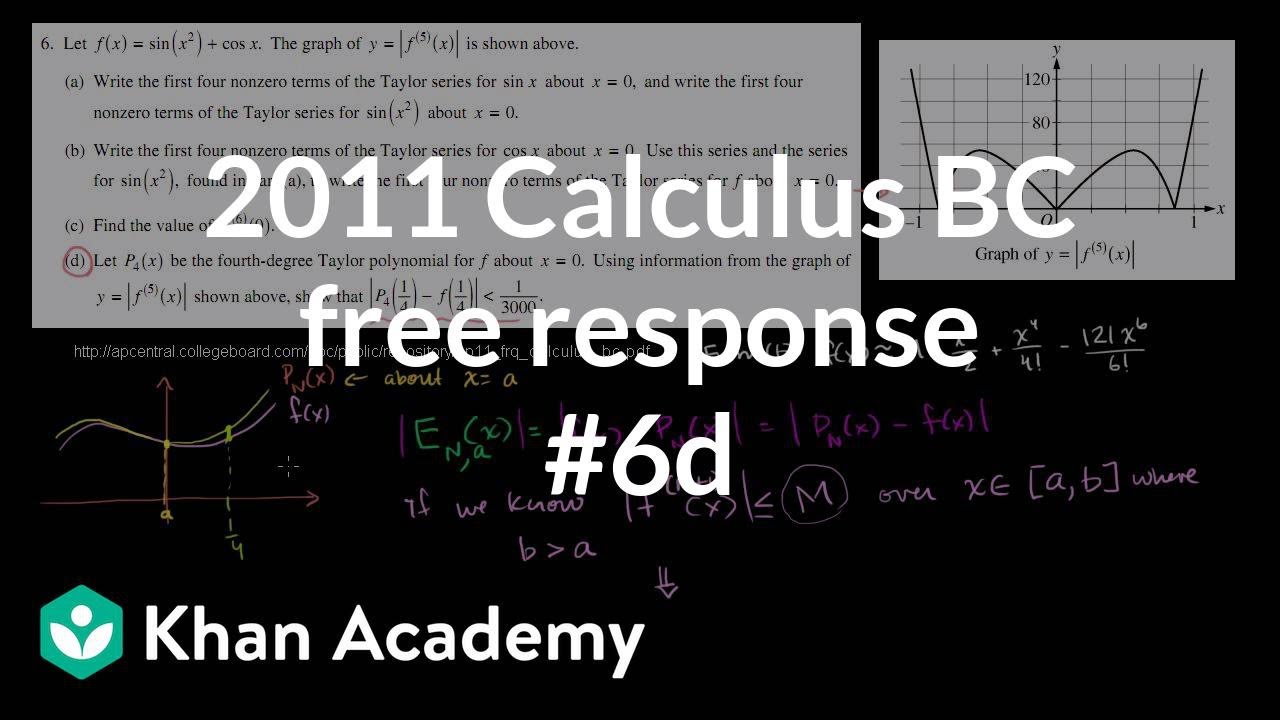
2011 Calculus BC free response #6d | AP Calculus BC | Khan Academy

Taylor polynomial remainder (part 2) | Series | AP Calculus BC | Khan Academy

Review of Lagrange Error Bound and Alternating Series Error for the BC Calculus Exam

Related Tags

Lagrange Error Bound Taylor Polynomials Maclaurin Polynomials Calculus Concepts Approximation Accuracy Mathematical Analysis Function Approximation Z Value Significance Math Education Advanced Math Topics