Lecture 14: Location, Scale, and LOTUS | Statistics 110
TLDRThe video script delves into the intricacies of the standard normal distribution, denoted as Z, and its properties. It covers the probability density function (PDF), cumulative distribution function (CDF), mean, and variance, highlighting that the mean of Z is 0 and the variance is 1. The讲师 (instructor) discusses the concept of moments, emphasizing that all odd moments of the standard normal distribution are zero due to symmetry. The general normal distribution is introduced as X = μ + σZ, where μ is the mean (or location) and σ is the standard deviation (or scale). The讲师 demonstrates how to derive the PDF of the general normal distribution using standardization and the properties of variance. The script also touches on the properties of variance, explaining its calculation and the common mistake of omitting the square when multiplying by a constant. The讲师 further explains the variance of the sum and difference of independent normal random variables and introduces the empirical rule (68-95-99.7% rule) for normal distributions. The script concludes with a discussion on the variance of the Poisson distribution and a method for calculating the variance of the binomial distribution using indicator random variables and linearity. The讲师 also explains the Law of the Unconscious Statistician (LOTUS) for both discrete and general cases, providing an intuitive understanding of why it holds true.
Takeaways
- 👨🔬 The standard normal distribution, often denoted as Z, has a probability density function (PDF) that is symmetrical around zero, and its cumulative distribution function (CDF) is represented by Φ.
- 🔨 Key properties of the standard normal distribution include a mean (E[Z]) of 0 and a variance (Var[Z]) of 1, highlighting its symmetry since any odd moment like E[Z^3] equals 0.
- ✅ When deriving distributions from the standard normal, transforming Z by adding a mean (μ) and multiplying by a standard deviation (σ) creates a new normal distribution X with mean μ and variance σ^2.
- ⚠️ The variance of a distribution does not change when a constant is added (Var[X+c] = Var[X]), but scales by the square of the factor when multiplied (Var[cX] = c^2 Var[X]).
- 📈 Discusses how variance properties differ from expectations: variance is not linear, and Var[X+Y] ≠ Var[X] + Var[Y] unless X and Y are independent.
- ➡️ The transformation of a normal variable X (X = μ + σZ) back to the standard normal form is called standardization (Z = (X-μ)/σ).
- 📝 Highlights the importance of the LOTUS (Law of the Unconscious Statistician), which is used to compute expectations of transformations of random variables without knowing their distribution.
- ✏️ Explains how to derive the PDF of a generalized normal distribution through differentiation of its CDF, demonstrating practical application of calculus in probability.
- 📉 Introduces the 68-95-99.7% rule for normal distributions, explaining how it describes the probability of a value falling within certain standard deviations from the mean.
- 📖 Emphasizes practical approaches to understanding distributions, such as exploring variances through summing independent variables, and stresses the importance of recognizing how operations affect variance and mean.
Q & A
What is the standard notation for the cumulative distribution function (CDF) of the standard normal distribution?
-The standard notation for the CDF of the standard normal distribution is capital Phi (Φ).
What is the mean of a standard normal random variable Z?
-The mean of a standard normal random variable Z is 0, which is evident due to the symmetry of the distribution around the y-axis.
How is the variance of a standard normal distribution calculated, and what is its value?
-The variance is calculated using integration by parts, and for a standard normal distribution, it equals 1.
What is the expected value of Z cubed for a standard normal random variable Z?
-The expected value of Z cubed is 0 because it is an odd function, and by symmetry, all odd moments of the normal distribution are 0.
What is the term used to describe the property that all odd moments of the normal distribution are zero?
-This property is referred to as the 'third moment' in the context of moments of a distribution.
How is the general normal distribution defined in terms of the standard normal distribution?
-The general normal distribution is defined as X = μ + σZ, where μ is the mean (or location) and σ is the standard deviation (or scale), and Z is a standard normal random variable.
What is the effect of adding a constant (mu) to a normal random variable on its variance?
-Adding a constant (mu) to a normal random variable does not change its variance. The variance remains the same because variance is unaffected by changes in location.
How does multiplying a normal random variable by a constant (sigma) affect its variance?
-Multiplying a normal random variable by a constant (sigma) results in the variance being multiplied by the square of that constant (sigma squared).
What is the rule of standardization for converting a general normal random variable X to a standard normal random variable Z?
-The rule of standardization is Z = (X - μ) / σ, where X is a normal random variable with mean μ and standard deviation σ, and Z is the resulting standard normal random variable.
What is the 68-95-99.7% rule for the normal distribution, and what does it signify?
-The 68-95-99.7% rule states that for a normal distribution, approximately 68% of the data falls within one standard deviation of the mean, 95% falls within two standard deviations, and 99.7% falls within three standard deviations.
How is the variance of a Poisson random variable with parameter lambda derived, and what is its value?
-The variance of a Poisson random variable is derived using the law of the unconscious statistician (LOTUS) and is found to be equal to lambda, the parameter of the Poisson distribution.
What is the variance of a binomial random variable with parameters n and p?
-The variance of a binomial random variable is npq, where q = 1 - p, and both n and p are the parameters of the binomial distribution.
Outlines
📚 Introduction to Standard Normal Distribution
The paragraph begins with a review of the standard normal distribution, denoted as Z, which has a mean of 0 and a variance of 1. The cumulative distribution function (CDF) of the standard normal is symbolized by the capital Phi and cannot be expressed in closed form. The properties of the standard normal are discussed, including its mean and variance, and the fact that all odd moments (E[Z^n] for odd n) are zero due to symmetry. The concept of moments is introduced, and the importance of symmetry in understanding the distribution is highlighted. The general normal distribution is then introduced as X = μ + σZ, where μ is the mean (or location) and σ is the standard deviation (or scale).
🔍 Properties of Variance and Transformations
This section delves into the properties of variance, emphasizing that variance is not linear and cannot be negative. It explains how adding a constant to a random variable does not affect its variance, but multiplying by a constant c results in the variance being multiplied by c^2. The importance of squaring the constant when applying it to the variance is stressed to avoid computational errors. The paragraph also clarifies that the variance of a sum of two random variables is not simply the sum of their variances unless the variables are independent. The concept of standardization for normal distributions is introduced as X = μ + σZ, and the reverse process is also explained.
🧮 Deriving the PDF of the General Normal Distribution
The paragraph focuses on deriving the probability density function (PDF) of a general normal distribution with mean μ and variance σ^2. It uses the standardization technique to transform the random variable X into a standard normal Z, and then applies the chain rule from calculus to find the derivative of the CDF, which yields the PDF. The process is demonstrated to be straightforward once the PDF of the standard normal distribution is known. The concept of the 68-95-99.7% rule is introduced as a rule of thumb for the normal distribution, indicating the probability of a normal random variable falling within a certain number of standard deviations from the mean.
📉 Variance of the Poisson Distribution
The discussion shifts to the Poisson distribution, which is characterized by having a mean and variance both equal to lambda (λ). The process of finding the variance involves using the moment-generating function (MGF) of the Poisson distribution and applying derivatives to find E[X^2]. The sum of λ^k/k! is derived using the Taylor series expansion of e^λ, and the variance is ultimately found by subtracting the square of the mean from E[X^2]. The properties of the Poisson distribution are highlighted, including the fact that the mean equals the variance.
🎯 Variance of the Binomial Distribution
The paragraph tackles the calculation of the variance for a binomial distribution. It outlines three potential methods for finding the variance: a direct but tedious calculation using the binomial PMF, an easy method that relies on the variance of independent sums (which is not yet proven), and a compromise method using indicator random variables. The compromise method involves squaring the binomial expression, summing over all terms, and then applying expected values to simplify the expression. The result is the variance of the binomial distribution, which is given by np(1-p), where n is the number of trials and p is the probability of success in each trial.
🧩 LOTUS and Its Proof for Discrete Random Variables
The final paragraph provides an explanation for the Law of the Unconscious Statistician (LOTUS), particularly for discrete random variables. LOTUS states that the expected value of a function of a random variable can be computed as a sum of the function times the probability mass function (PMF) without first determining the distribution of the function. The proof involves considering the sum over all possible values of the random variable and grouping them into 'super pebbles' based on their values. The double sum representation is used to show that the expected value can be computed by first summing over all values of the random variable and then summing over the corresponding probabilities, leading to the conclusion that LOTUS holds true.
Mindmap
Keywords
💡Standard Normal
💡PDF (Probability Density Function)
💡CDF (Cumulative Distribution Function)
💡Variance
💡Moment
💡LOTUS (Law of the Unconscious Statistician)
💡Standardization
💡General Normal Distribution
💡Independence
💡68-95-99.7% Rule
Highlights
The standard normal distribution, often denoted as Z, has a mean (E[Z]) of 0 and a variance of 1.
All odd moments (E[Z^n] for odd n) of the standard normal distribution are zero due to symmetry.
The even moments of the standard normal distribution can be computed using integration techniques.
The concept of 'moments' in statistics refers to the expected values of powers of a random variable.
Minus Z is also standard normal, highlighting the symmetry of the standard normal distribution.
General normal distribution X can be expressed as X = μ + σZ, where μ is the mean and σ is the standard deviation.
The mean and variance of a general normal distribution X are μ and σ^2, respectively.
Standardization of a normal variable X is achieved by subtracting the mean and dividing by the standard deviation (X - μ) / σ.
The PDF of a general normal distribution can be derived from the standard normal PDF using standardization.
The variance of a scaled random variable is the square of the scaling factor times the original variance.
The sum of independent normal random variables is itself normal, with a mean equal to the sum of the means and variance equal to the sum of the variances.
The empirical rule (68-95-99.7% rule) provides a quick way to estimate the probability of a normal variable falling within certain standard deviation ranges.
The variance of a Poisson random variable with parameter λ is equal to λ, which is also its mean.
The binomial variance can be calculated using the formula npq, where n is the number of trials, p is the probability of success, and q = 1 - p.
Linearity of expectation (LOTUS) allows for the computation of the expected value of a function of a random variable without needing the distribution of that function.
The proof of LOTUS for a discrete sample space involves grouping and ungrouping pebbles (outcomes) in a way that maintains the average value.
The double sum technique used in the proof of LOTUS rearranges terms to show that the expected value of a function of a random variable can be computed directly from the random variable's distribution.
Transcripts
So last time we were talking about standard normal, right?
Normal zero one.
So just a few quick facts that we proved last time.
So our notation is, traditionally it's often called Z, but
I'm not saying Z has to be standard normal.
Or you have to call standard normal Z, just we often use letter Z for that.
If Z is standard normal, then first of all, we found its PDF, right?
We figured out the normalizing constant,it's CDF.
It's CDF you can't actually do in closed form,
so therefore it's just called capital Phi.
That's just the standard notation for the CDF.
We computed the mean and the variance last time.
Remember, the mean E of Z = 0.
That's just immediate by symmetry.
Then we also did the variance.
Variance equals in this case the variance is E of Z squared equals 1.
Cuz variance of E of Z squared minus E of Z squared the other way,
but that's 0, so that's one.
That we computed last time using integration by parts, so
we did that last time.
And if we wanted, this is by the way it's called the first moment, second moment.
If we wanted E of Z cubed, this we didn't talk about last time.
That's gonna be 0 again.
Because, I'll just write down what it would be.
By LOTUS, we would have the integral minus infinity, infinity 1 over root 2 pi,
E to the minus Z squared over 2 dz.
This integrates 1, that would be just integrating the PDF.
And LOTUS says if we want E of Z cubed, we just stick in a Z cubed here.
If we just wanted to do E of Z, we'd put Z, if we want E of Z cubed,
we'd put Z cubed, that's LOTUS.
But this is just equal to 0, because this is an odd function, again.
So we talked about that in this case, but the same argument would apply here for
Z cubed.
Similarly, for any odd power here, 5, 7, and so on, we'll immediately get 0.
So this is called the third moment.
At some point later in the semester we can talk about where does the word moment
come from.
But that's just that's just terminology for that that's called the third moment.
E of Z cubed that would be called the second moment first moment then and so on.
Okay so in other words,
by symmetry we already know that all the odd moments of the normal are 0.
The even moments well,
we have this the second one if we wanted E of Z to the fourth.
Well it's going to be the integral except put Z to the fourth instead of Z cubed,
then that's not such an easy integral anymore,okay?
And it's not an integral that you need to know how to do it at this point,
we'll probably come back to how to do things like that later,
not before the midterm though.
But at least you should immediately know LOTUS that you could
write down the integral for E of Z to the fourth, it's just that
happens to be an integral that I don't expect that anyone could do right now.
But at least you could write down the integral, okay?
Odd moments though, you just immediately get 0 by symmetry, no integrals needed.
Okay so I was talking about symmetry, let me just mention symmetry one other way
which is that minus Z is also standard normal.
And that's just another way to express the symmetry of it.
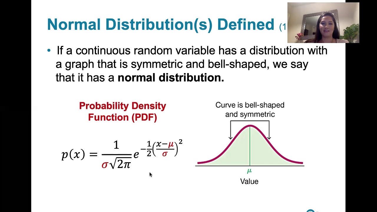
That is, the PDF is this bell curve that's symmetrical about 0.
So if you flip, this flips between plus and minus, right.
Just flipping the sign, that changes the random variable,
it makes a positive into negative, makes negative into positive.
But it does not change the distribution, that's what the symmetry says.
So you can either just see this by symmetry or you could compute the PDF of
this by first find the CDF, then find the PDF, and you'll see that that's true.
That's a very useful fact., it's always useful looking for symmetries.
Okay, so this is just stuff about the standard normal.
But now we wanna introduce what happens with normal
where this is not necessarily 0, 1, okay?
So this is the general normal.
We say that X, if we let X equal mu plus sigma Z
where mu is any real number and
we would call that the mean cuz that's going to be the mean.
But we would also call that the location.
Because we're just adding a constant, it means a shift in location.
We're not changing what the density looks like by adding mu,
we're just moving it around left and right.
And sigma is any positive number, mu could be negative,
sigma has to be positive, and that's called the standard deviation.
Remember standard deviation we defined as the square root of variance.
So sigma is the standard deviation but we also call that the scale
because we're just rescaling everything by multiplying by a constant.
So that's gonna effect if you draw one of the density,
it's gonna effect how wide or how narrow that curve is.
It still has to integrate to 1, so you can't just make it really big and wide and
suddenly you made the area blow up.
You also have to make sure that you multiply by a normalizing constant so
it still integrates to 1, but you can still make it more wide or more narrow.
Okay then we say Then we say X is normal
with mean mu and variance sigma squared.
So those are the two parameters.
So the reason most books would do this a little bit differently and
start by writing down the PDF of this.
But this is a more useful and more insightful way to think about it,
where we're saying there's just one fundamental basic normal distribution.
That's what we call the standard normal.
Once we understand the standard normal we can easily get any other normal
distribution we want just by multiplying by a constant adding a constant.
So it's reducing everything back down to the standard normal.
That's really useful to always keep that in mind instead of just
looking at ugly formulas, okay?
So let's actually check that this has the desired mean and variance.
So obviously the expected value of X just by linearity with mu plus
sigma expected value of Z is 0, so that's just mu, just immediate from this.
For the variance, Then we need to talk
a little bit more about what happens, what are the properties of variance.
So I'll come back to this in a minute.
First, let's just talk a little bit more in general about variance.
We did a quick introduction to variance before but
we should go a little bit further.
So remember, there's two ways to write variance.
The definition is to subtract off the mean, square it,
the average distance squared of X from its mean.
But we also showed that can also be written as E(X) squared, this way,
minus E(X) squared the other way, okay?
Now in particular, if we had the variance of X plus a constant, intuitively,
if we just add a constant we're not changing how variable X is, right?
So intuitively that should be the same as the variance of X.
And you can see that immediately from this first formula because You replace by x by
x + c, and the mean also shifts by c by linearity, you get the exact same thing.
So that's immediate from this, so adding a constant has no effect on the variance.
Now if we multiply by a constant, then from either of these formulas,
just imagine sticking in a c here and a c here.
But the c comes out because of linearity again, but it's squared, then.
So the variance of a c times x is c squared times the variance of x.
And a common mistake is to forget the square here, but
that really messes things up, so variance is coming out with the square.
And an easy way to see that is, if c is negative, this is still valid.
But if you forgot to write the square here, you would get a negative variance.
If you ever get a negative variance, that's very, very bad,
variance cannot be negative.
So anytime you compute a variance, the first thing you should check is,
is the thing I wrote down at least non-negative?
And the only case where it could be 0 is if it's a constant,
so it's always greater than or equal to 0.
And variance of X = 0 if and
only if X is a constant with probability 1.
P of X = a = 1 for some a, that is,
with probability 0, something bad could happen.
But with probability 1, it always equals this constant a.
So that would have variance 0 because the stuff
with probability 0 doesn't affect anything, so essentially it's a constant.
If it's not a constant, the variance will be strictly positive.
Okay, so that's the variance of a constant times x, and then just one other factor
about, we'll do a lot more with variance like after the midterm.
But only one other thing to point out for now is that variance,
unlike expected values, variance is not linear.
So variance of x + y is not equal to variance x plus variance of y.
In general, it may be equal, but it's not necessarily equal, so
actually, it violates both of the linearity properties.
If it were linear, we would want constants to come out as themselves, and
here it comes out squared.
And we can't say the variance of the sum is the sum of the variances.
It is equal, we're not gonna show this until later,
we'll show this at sometime after the midterm.
It is equal if x and y are independent, but remember,
linearity holds regardless of whether the random variables are independent or not.
So if they're independent, it will be equal, we'll show that later, but
in general, they're not equal.
And one quick example of that would be, what if we look at the variance of x + x?
All right, that's an extreme case of dependence, that's when x,
it's actually the same thing, right?
Well, the variance of x + x Is the variance of 2x,
which we just said is 4 times the variance of x.
So if this were true, if this were equal, we would get 2 times the variance of x.
And this says we get 4 times the variability, not 2 times the variability,
but that's just a simple example of that.
But that's also a common mistake that I've seen before when students
are dealing with, in the past I've asked questions either on homeworks or
exams where we have something like 2x.
And a lot of students took the approach of, well, 2x is x + x.
Of course, that's valid, but then at that point,
they made the mistake of replacing x + x by, let's say, x1 + x2.
Where those are IID, with the same distribution as x.
That's completely wrong because x is not IID with itself.
It's extremely dependent and then somehow replacing it by independent copies,
then it doesn't work.
So I'm telling you to be careful of this,
just keeping track of dependents versus independents.
Here they're extremely dependent, and so that's why we got this 4 here.
And I think, intuitively, that should make some sense, right?
If this was like x1 and x2 and
they're independent, then the variabilities just add.
Here, they're exactly the same, so
that magnifies the variability, okay.
So that's a few quick notes about variance, so
now coming back to this for the normal case.
We just saw that adding mu does nothing to the variance, multiplying by sigma.
Then it comes out as sigma squared, that's sigma squared times the variance of z.
Well, that's just sigma squared, okay, so that confirms that
when we write this, this is the mean and this is the variance.
So those are the two parameters of the normal distribution.
Ane whenever you have a normal distribution,
you should always think about reducing it back to standard normal.
So we could also go the other way around, and I don't need much space for this.
Because this is just, I'm just gonna solve this equation for z, so
if we do it the other way, solve for z.
z equals x minus mu over sigma, very easy algebra,
that's called standardization.
So standardization says, I'm just going the other direction here.
I was starting with the standard normal, and
we can construct a general normal this way.
Now what if we wanted to go the other way, we started with x,
which is normal mu sigma squared.
Subtract the mean divided by the standard deviation,
and that will always give us a standard normal.
So that process is called standardization, it's very, very useful, it's simple,
right, just subtract the mean divided by the standard deviation.
And yet sometimes students get confused about it, or
divide by the variance instead of dividing by the standard deviation, or
just don't think to do it in the first place.
So that's why I'm emphasizing that, it's a simple but useful transformation.
Okay, so as a quick example of how we use that,
let's derive the PDF of the general normal.
Find PDF of normal mu sigma squared, well,
one way to find it is to look it up in a book.
But that doesn't tell you anything, that's just like a formula in a book.
So what we want to understand is, assuming that we already know the PDF of
the standard normal, how can we get the PDF of the non-standard normal?
In a way, that's easy, without having to memorize stuff, okay,
so let's call this x again, so let's find the CDF first.
So by definition, this is just good practice with CDFs.
Everyone here should make sure that you're good at CDFs and PDFs and PMFs.
And that just takes practice, so this is just some simple practice with that.
By definition, the CDF is this, and
now I just told you that a useful trick is to standardize, so let's standardize this.
It's the same thing as saying X minus mu over sigma is less than or
equal to lowercase x minus mu over sigma, right.
Sigma is positive, so it doesn't flip the inequality to do that, so
I standardized it.
The reason I standardized it was because now,
this thing on the left is standard normal.
So by definition, this is just the CDF of the standard normal evaluated here.
So by definition, we immediately know that's just
capital phi of x minus mu over sigma, now to get the PDF,
To get the PDF we just have to take the derivative of the CDF.
That's just the chain rule right, because this capital phi is the outer function and
then we have this inner function here so
it's just the chain rule from basic calculus.
It's the derivative of the outer function evaluated here,
times the derivative of the inner function.
The derivative of this inner function is just 1 over sigma, right,
cuz 1 over sigma times x.
So we are gonna get a 1 over sigma, and then we are gonna get the derivative of
this the derivative of capital phi is just the standard normal PDF, right?
And it says evaluated here, so I'm just gonna write down the standard normal PDF,
and I'm gonna evaluate it at x- mu over sigma.
And that's it, we're done.
So it should be a very,
very quick calculation in order to be able to do that.
And as another quick example.
Let's say over here in the corner, we said what happens,
z is standard normal, what happens to -z?
Let's also ask the question of what happens to -x?
Well, you could work through a similar calculation, but
I think the neatest way to think of it is, we're thinking of x as mu + sigma z.
So -x- mu + sigma times -z.
But -z is standard normal.
So this is just of the form some
location constant plus sigma times the standard normal.
So we immediately know that's normal -mu sigma squared.
Which again, makes sense intuitively, because we put a minus sign, so
we put a minus sign on the mean.
We do not put a minus sign on the variance,
because variance can't be negative, so the variants stay sigma squared.
So you could do a calculation for this, but
this is just immediate from thinking of x in terms of the standard normal.
So this is the easiest way to do this, okay?
And a useful fact just to know, but we'll prove this much later in the course.
Later we'll show that if x1,
let's say xj is normal mu j,
sigma j squared, and they're independent.
Let's say for j equals 1 to 2.
Then, x1 + x2 is normal, mu1 + mu2
sigma 1 squared + sigma 2 squared.
So that's something we need to prove, and we'll do that much later.
The sum of independent normals is normal, but the reason I'm mentioning it now is
just let's think about what happens to the mean and variance.
By linearity, we know that the mean would have to be mu1 + mu2.
Variance, this is something else we'll prove later.
In the independent case we can just add up the variances, so
it's juts sigma1 squared + sigma2 squared.
Now what if we looked at x1- x2?
I'm mentioning this now,
because I can't even count the number of times when I've seen the mean is mu1- mu2.
That's just linearity again.
I can't even count the number of times I've seen
students write that the variance is sigma1 squared- sigma2 squared.
Well, first of all that could be negative, so that doesn't make any sense.
And secondly, any time you see a subtraction you can really think of that
as adding the negative of something, right?
So this is + of -x2.
And -x2 still has variance sigma2 squared, so the variance is still add.
That's just a useful fact to keep in mind, we'll prove it later.
But I'm mainly talking about right now just in terms of what happens to
the mean and variance.
Later we'll see why are they still normal.
That's just one very useful property of the normal.
So let's just do a lot of things without leaving the realm of normality, right?
If you added two of them and then it somehow becomes some completely different
distribution, it's gonna be hard to work with.
So that's a very nice property of the normal.
Okay, one other fact about the normal
that's just like a rule of thumb for the normal.
Because of the fact that you can't actually compute this function,
capital phi other than by having a table of values.
Or a computer that, or
a calculator that specifically knows how to do that function.
You can't do it in terms of other functions,
it's useful to just have a few quick rules of thumb, so
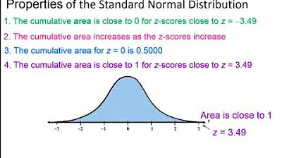
there's something called the 68- 95-99.7% rule.
And I don't know who named it that, but at the first time I heard of this
that's the stupidest name for a rule that I have ever heard of.
However, then I always remember that, so actually it works very well.
It simply says it's just the three simple numbers telling us
how likely is it that a normal random variable will be a certain
distance from its mean measured in terms of standard deviation.
So this says that, if x is normal,
then the statement is that the probability
that x is more than 1 standard deviation from its mean.
So notationally we would just write it like that.
But intuitively, that's just saying what's the chance that it falls more than 1
standard deviation, right?
That's 1 standard deviation.
This would say the distance is more than 1 standard deviation away from the mean.
Well, I was actually right the other way.
The probability that x is within 1 standard deviation of
its mean is about 68%.
The chance that x is within 2 standard deviations of its mean is about 95%.
And the chance that it's same with 3 standard deviations is about 99.7%.
So, in other words, it's very common for
people in practice to add and subtract 2 standard deviations.
What that's saying is for the normal, that's gonna have 95% chance of so,
let's say you got a bunch of observations from this distribution independently.
We would expect about 95% of them are gonna be within 2 standard
deviations of the mean, 99.7% within 3.
So you can convert these statements into statements about capital phi which is good
practice while just making sure you understand what capital phi is.
But basically, this is just a few values of capital phi just written in kind of
a more intuitive way.
Okay, so that's all for the normal distribution.
So the main thing left to talk more about is LOTUS, and
a couple examples of LOTUS and using LOTUS to compute variances.
For example,
we proved that the variance of the Poisson is Poisson lambda has, sorry.
We proved that the mean of a Poisson lambda is lambda.
We have not yet derived the variance of a Poisson lambda.
So that's definitely something we should do.
So, okay.
So let's do the variance of the Poisson.
And that will also give us a change to understand more,
what's really going on with LOTUS?
Why does LOTUS really work?
So suppose we had a random variable such as the Poisson, but
right now I'm just thinking in general.
A random variable who's possible values are zero, one, two, three, and so on.
So let's call our random variable x.
And x can be 0, 1,
2, 3, etc, okay?
And suppose that its pmf.
To say what the pmf is I just need to say what's the probability of,
0 let's call that P0 probability of 1, P1, P2, P3.
So all I did here was write out the pmf,
just stringing it out as a sequence, right?
But that's just specifying the pmf and
I'm calling them pj is the probability that x equals j.
Now to figure out variance we need to study x-squared, right?
So let's look at x squared.
So 0-squared is 0, 1-squared is 1, 2-squared is 4,
3-squared is 9, and we keep going like that.
From this point of view, it should be easy to see what we should do.
Because E(x), remember for
a discrete random variable E(x) is the sum of x times the pmf.
Now here we want E(x-squared),
but notice that the probability that x-squared equals say 3-squared
is just the probability P3 of being in this column here, right?
So the probabilities didn't change, and
we could just still use x-squared times the probability that x = x, right?
Because when an x-squared takes on these possible values
with these same probabilities.
That's what LOTUS is saying, so it's pretty intuitive in that sense.
The case that you have to think more about is the case where this function is not
1 to 1.
So now squaring is not 1 to 1 in general.
If I had had negative numbers, then you would have duplicates here and
you would have to sort that out.
What LOTUS says is even when you have those duplications, this still works.
That I think is a little less obvious,
if you think about it you can see why it's true, but it's not completely obvious.
In this case, because we're not non-negative anyway,
this is one to one and then it just immediately true, okay?
But LOTUS this is saying, no matter how complicated your function is,
something kind of this flavor still works,
regardless of whether you have duplications.
So now we're ready to get the Poisson variance.
So this is just in general if you
have a random variable non-negative integer values.
Now let's look at the specific case of Poisson lambda and
we want to find E(x) squared.
And according to LOTUS we can just write that as the sum k = 0 to
infinity k-squared E to the minus lambda,
lambda to the k over k factorial, that's the pmf.
So we have to figure out how to do this sum,
and this looks like a pretty unfamiliar sum.
I mean my first thought when I see this would be, well this is k times k and
we can cancel and get a k minus one factorial here.
And there's nothing wrong with doing that but
it's still kind of annoying because we still have k-squared up here.
When we were just planning the mean, then we just had a k and
we cancelled it and things are nice.
But now we have a k-squared, it's more annoying, okay?
So here's another method for dealing with something like that.
The general method is start with what we know, right?
So what we know how to do is the Taylor series for e to the x.
Hopefully you all know that by now, we keep using it over and over again.
The sum, I'll write it in terms of lambda.
The sum of lambda to the k over k factorial.
Is e to the lambda, and this is valid for all real lambda, even for
imaginary numbers, complex numbers, this is always true, always converges.
Now if I wanna get a k in front,
then a natural strategy would be to take the derivative of both sides.
Well that's pretty nice right,
because the derivative e to the lambda is e to the lambda.
The derivative of the left-hand side,
I'll start the sum at 1 now because at 0 it's 0.
So we have k lambda to the k -1 over k factorial.
I just took the derivative of both sides.
I exchanged the derivative and the sum,
which is valid under some mild technical conditions.
Now we're getting closer, but we still only have a k, not a k squared, okay?
So my first impulse would be, take a derivative again,
that's slightly annoying cuz then I'd get a k-1 coming down, I want a k, not a k-1.
So to fix that, all we have to do is multiply both sides by lambda, okay?
So, just put lambda on both sides.
So I call that replenishing the lambdas.
We just replenish it, that we have a lambda there.
I'll write it again, k equals one to infinity.
K, lambda to the k over k factorial equals lambda e to the lambda.
We've replenished our supply of lambda's,
now we can take the derivative again and we have what we want.
Okay, so I take the derivative a second time and
k = 1 to infinity, take the derivative again, now it's k-squared.
Lambda to the k- 1 over k factorial.
Well now we have to use the product rule, the derivative of lambda, e to the lambda
is lambda e to the lambda plus e to the lambda by the product rule.
Which we can factor out as e to the lambda times lambda + 1.
Okay, well that's exactly the sum that we needed.
Cuz this e to the minus lambda comes out, so
this is e to the minus lambda, e to the lambda, lambda + 1.
I'm missing some, is there another lambda somewhere?
Lets see, we have to replenish it again.
Just put a lambda.
Okay, so here we have lambda to the k- 1, there we want lambda to the k.
So its replenish again, then there is another lambda there, okay.
I'm just bringing this k- 1 back to being lambda to the k, right?
So that's just lambda squared + lambda.
And now we have the variance.
So the variance of X equals this thing,
lambda squared plus lambda minus the square of the mean,
which is lambda squared equals lambda.
So this course is not really about memorizing formulas, but
that's one that's very easy and useful to remember.
The Poisson lambda has mean lambda, and has variance lambda.
So that's kind of a strange property if you think about it.
That the mean equals the variance, it's a little bit,
maybe it would seem more natural if the mean equal the standard deviation or
something like that, because then those are kind of in the same scale.
But Poisson, it doesn't actually have units.
Poisson is just counting numbers of things, so
it doesn't have that some dimensional interpretation.
So, yeah, I wanted to also mention that about standardization as well.
Another reason this thing is really nice to work with in the normal is if
you think of normal as being a continuous measurement in some unit,
it could be a unit of length, time, mass, whatever.
If x is measured in whatever unit you want,
let's say it's time measured in seconds, then that's seconds
minus seconds divided by seconds, the seconds cancel out.
That means this is a dimensionless quantity, which is part of what's making
this standardization, it's kind of making it more directly interpretable
instead of having to worry about whether you measured it in seconds or years.
So if we started with one measurement in seconds and one measurement in years and
standardized both of them, we get the same thing.
The same measurement in different units.
So that's a nice property of that.
Okay, so that's the variance of the Poisson.
We haven't yet gotten the variance of the binomial, so I'd like to do that.
There's an easy way and a hard way.
Well, except the hard way I don't think, actually sorry,
there's three ways to do it.
There's a really easy way that we can't do yet
because we haven't proven the necessary fact.
There's an easy way that we can do, so that's what I'm gonna do.
And then there's an annoying way, which we're not gonna do.
The annoying but direct is we want the variance of a binomial.
We wanna find the variance.
The most direct obvious way to do this would be to use lotus to get E(x squared)
which would mean you would have to write down something like this,
except here we wrote the Poisson PMF.
Instead you'd have to write n choose k, p to the k, whatever,
the binomial PMF, right.
And then you'd have to do that sum.
And you can do it, but that's pretty tedious.
And you have to figure out how to do that sum and do a lot of algebra.
Okay, so that's the way I don't wanna do it.
The easiest way to do it would be using this fact here.
Which is that the variance of a sum of independent things is the sum of
the variance, if they're independent, right.
That's if, okay.
So the easiest one, we haven't proven this yet so
this is not valid to do it at this way right now but just kinda foreshadowing.
We can think of the binomial,
we've emphasized the fact that we can think of a binomial as the sum of n
independent Bernoulli p.
So once we prove this fact, that's applicable.
So all we have to do is get the variance of Bernoulli p,
which is a really easy calculation cuz the Bernoulli is just zero one,
so that's a very very easy calculation.
To get the variance of a Bernoulli p and multiply by n,
that's the neatest way to do it.
You can do it that way in your head once we get to that point, okay.
Now here's kind of the compromise method which is also just good practice with
other concepts we've done, especially indicator random variables.
So I'm still going to use the same idea of
representing x as a sum of Iid Bernoulli p.
So I'll write them as I1 plus blah, blah, blah, plus In,
just to emphasize the fact that they're indicators, I for indicator.
Where Ijs are Iid Bournulli p, right.
So we've been doing this many times already.
That's just an indicator of success on the jth trial, add up those and
we get a binomial.
Okay, so now if we want the expected value of x
squared, Let's just square this thing.
Let's actually not do the expected value yet.
We'll just square it then take the expected value.
So just square this thing.
Well you know you do i1 squared and just square all the things, right.
So it's i1 squared plus blah blah blah plus In squared plus,
but as you know we get a lot of cross terms, right.
Your imagining this big thing times itself, so every possible cross term,
each one twice, you have 2I 1I 2 and 2I 1I 3 and so on.
All possible cross terms and each cross term has 2 in front.
Just like when you square x+y, you get x squared + y squared + 2xy.
We get all these cross terms.
It doesn't matter what order we write them in.
Maybe we've ordered them in this way.
So that's the last one.
It doesn't matter the order.
Okay, so it's all the cross terms.
That looks pretty complicated.
But it's actually much simpler than it looks.
Now let's take the expected value of both sides, use linearity.
Of the same, this is a good review example as well.
We're using the same tricks, symmetry, indicator, random variables, and
linearity.
Each of these, these are Iid.
So by symmetry, this is just n times anyone of them.
So let's just say nE(1 squared).
That's just immediate by symmetry, right.
So we don't have to write that big sum, just n times one of them.
And how let's just count how many of these,
well there's n choose two cross terms, right.
Because for any pair of subscripts we have a cross term.
So it's really just 2(n choose 2), and then just take one of them for
concreteness, let's say E(I1I2).
Now this is even nicer, well it definitely is looking better.
But this is even better than it looks because I1 is either just 1 or 0.
If you square one you got one, if you square zero you got zero.
So I1 squared is just I1.
So E(I1), that's just the expectorate of Bernoulli p is p.
So that's just np+n
choose 2 is n times n-1 over 2, so the 2s cancel.
So this is really just n(n-1).
Now let's think about this indicator random variable.
Well I called it an indicator random variable,
well actually it's a product of indicator random variables.
But actually a product of indicator random variables is an indicator random variable.
This thing here is the indicator of success on both the first and
the second trial, right.
Because if you think of multiplying two numbers that are zero and one, you
get zero if at least one of these is zero, you would get one if they're both one.
So that's the indicator of success on both.
So it's a product but it's actually just one indicator.
Success on both trials, number 1 and 2.
So its expected value is just the probability of that happening.
That probability of success on both the first trial and
the second trial, because the trials are independent, is just p squared.
Okay, so that's just, so
what we just computed is the second moment of the binomial.
That's np+, if we multiply that
np+n squared p squared-np squared, right.
Now to get the variance all we have to do is subtract, The square of the mean, okay.
So we showed before that a binomial np has mean n times p.
So if we square that, that's this term n squared p squared, so that cancels.
So we're just canceling out this middle term and
we just have np- np squared = np (1- p).
Which we would often write
as npq with q = 1- p.
So binomial variance is npq.
So that's just a good review of indicator of random variables and all of that stuff.
So now we know the variance of the Poisson,
the normal, the uniform, the binomial.
For the geometric, it's kind
of a similar calculation, we did the mean of the geometric in two different ways.
The flavor of the calculation is similar to this except we have a geometric series
instead of the Taylor series for e to the x.
So I don't think it's worth doing that in class.
So in general hypergeometric, let's talk a little bit about hypergeometric,
that's pretty nasty.
In the sense that in the hypergeometric,
we could write it as a sum of indicator random variables.
We're imagining we're drawing balls one at a time and, or
picking elk one at a time and success is getting a tagged elk.
But the problem is that they're not independent.
So as far as the mean is concerned we still use linearity.
For the variance it's more complicated.
So we'll worry about the variance of a hypergeometric after the midterm.
That's more complicated.
But for the binomial this is really, well, actually we could still.
Here I didn't actually use the factor there independent cuz I was just using
linearity.
So you could use a similar approach, so actually you could do it this way, but
it would be too tedious to do it like on a midterm or something.
But you could square it, if these are dependent well, you can still work out
the probability that the first two elk that you pick are both tagged.
You could do that without too much trouble.
But it's pretty messy looking.
All right, so that's variance, and I guess the last thing
to do is just to explain more about why is LOTUS true?
And the basic proof of that is actually kind of
conceptually similar to how we proved linearity.
So we're trying to prove LOTUS, and I'm only gonna prove it for a discrete.
Let's say discrete sample space.
That's the case where I'm imagining finitely many pebbles.
In the general case the ideas are not essentially different.
It's just that we kind of need to write down some fancier integrals and
use more kind of more technical math, but the concept is similar.
So this is enough to give you the idea.
So for discrete sample space, so the statement is that
the expected value, that's all we are trying to show,
is that the E(g(x)) can be written as the sum of g(x) P(X=x).
So right, we can use the PMF of x we do not have to first work
on figuring out the distribution of g(x).
That's all we are trying to do, so let's think about it.
Let's think about it as a sum of, sum over the other.
We could sum the other way around, sorry.
Let me say this a different way,
let me remind you of the identity that we use for proving linearity.
That was this group versus ungroup thing.
So what we have is two different ways to write a certain sum.
We could either write this thing, g(x)P(X=x) or we could write
it the other way, which is a sum over all s.
Each s, we're thinking of that as s in the sample space S.
So each little s is a pebble.
And if we're summing it up pebble by pebble,
then what we're doing is remember random variables are functions.
So, and g(x) just means we apply the function x then apply the function g.
So we're just computing g(x(s)),
that's just the definition times the mass of that pebble.
So.
If you stare at this equation long enough, and
we have five minutes left to stare at that equation, so that's plenty of time.
This is why LOTUS is true.
It's just a matter of understanding this equation.
So I'm gonna talk a little more about, how do you make sense of this equation?
This is the grouped case.
This is the ungrouped case.
Remember I talked about pebbles and super pebbles, ungrouped.
This says take each pebble, compute this function,
g of x of s, and you take a weighted average.
Those are the weights.
This says, first combine all of the pebbles that have
the same value of x into you know, super-pebbles.
A super-pebble means we grouped together all pebbles with the same x value,
not the same g(x) value, the same x value.
Group those together then average, you get the same thing.
So if I want to write that out in a little bit more detail.
One way to think of it is as a double sum, right?
Because we could imagine first summing over x.
I'm gonna break this sum up.
What I just explained to you was the intuition for why this is equal to this.
Because we're just grouping them together in different ways so
we changed the weights around, but as long as we changed the weights appropriately we
should get the same average.
That's the intuition.
But for any of you who wanna see more of an algebraic reason, justification for
that, the way to think of it is as a double sum.
So the double sum would be,
I mean to rewrite this says sum overall pebbles right?
But one way to think of that would be first sum over values of little x.
And then for each value of little x, sum over all pebbles,
s such that x(s) = x.
Because this is just a sum of a bunch of a numbers.
We can sum them in any order we want.
So I can rearrange them,
in this particular order where I'm saying first sum over the little x values, and
then group together, and sum over all the pebbles that have that value.
It's the exact same thing, I just reordered the terms.
So that's g(x(s)) times P(s).
Now let's just simplify this double sum.
The reason I wanted to write it as a double sum like this is that within this
inner summation X(s)=, so this thing is just g(x).
The cool thing is that g(x) does not depend on s so that comes out.
So we actually have the sum over x of g(x) times
the sum of what ever is left p(s).
And now so that's summed over all s such that s(x) = x.
And now we're done with the proof because this
sum here is just saying add up the masses of all the pebbles labeled x.
In other words, that's what I called a super pebble.
The super pebble, the mass is the sum of all
the masses of the little pebbles that form the super pebble.
That's p of, this is just practice,
this is going back to the very beginning of, events and what's a random variable.
That's just the event X = x.
We talked, what does it mean for big X to equal little x, right?
What does that equation mean?
That's an event.
That's this event that we have here.
Okay, so that's why that's true.
So that's why LOTUS is true.
Anyway that's all for now and Friday we'll review,
let me know if you have any suggestions for things to do on Friday.
Browse More Related Video
Elementary Statistics - Chapter 6 Normal Probability Distributions Part 1
6.1.3 The Standard Normal Distribution - Normal Dist. and Properties of the Standard Normal Dist.
Standard error of the mean | Inferential statistics | Probability and Statistics | Khan Academy
Variance and standard deviation of a discrete random variable | AP Statistics | Khan Academy

Visualizing the Binomial Distribution (6.6)

Elementary Stats Lesson #11
5.0 / 5 (0 votes)
Thanks for rating: